Thus, the development of XML-aware data mining techniques and query languages is also an important part of research. The frequency of a sequence S, denoted Freq(S,D), is the number of sequences S' in D such that S is a subsequence of S'.
Definitions
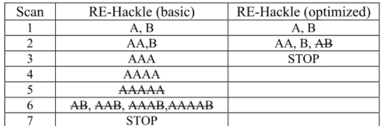
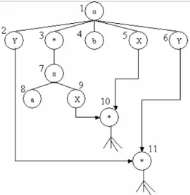
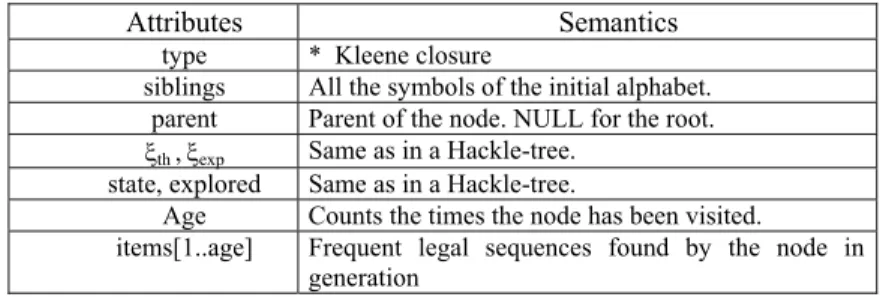
Sub-constraints are extracted from the initial RE-constraint: they correspond to the expressions of the derived phrase. A hackle-tree is an AST that encodes the structure of the canonical form of an RE-constraint.
The RE-Hackle Algorithm
Let us now discuss the processing of the Kleene closure nodes thanks to second-level alphabets. Using a second-level alphabet can boost the extraction of the Kleene closure, since the candidates are composed of sequences rather than simple symbols.
Optimization
The reconstruction of the extraction phase becomes more complex, as does the propagation of the violations and the candidate generation. The candidates from the nth age can be counted together with the frequent sequences of (n-1) age linked with the other siblings in the chain.
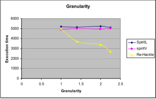
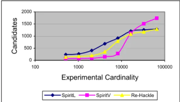
Experimental Results
If the parent of a closure is a concatenation that generates no regular sequence at a given iteration, then its sub-trees can be pruned immediately and exploration of the closure can be stopped. This way, when the nth age becomes empty, the concatenations of the (n-1)th age with the other siblings are available and no iteration is wasted.
Extension to RE-constraints with variables
If the result of a closure is empty, the node is immediately violated and pruned out of the X-tree. Note again that the duplication of the tree in an implementation can be avoided by smart indexing.
Conclusion
Iterate RE-Hackle(Tk, Vk[.], c) performs an RE-Hackle iteration on the Tk tree using the values from Vk[.] for instance variables. Takes all expressions containing variables and calculates the corresponding First and Last functions.
MR-SMOTI: A Data Mining System for Regression Tasks Tightly-Coupled with a Relational Database
The algorithm
This graph corresponds to the entire set of objects of interest in the relational database D (the target table T0). The functions optimal_split_refinement and optimal_regression_refinement take the selection graph G associated with the current node and consider every possible split and regression refinement.
The refinements
Furthermore, they can be applied to new instances stored in the relational database to predict an estimate of the unknown target attribute. The results of the Wilcoxon signed rank test on the accuracy of the induced multi-relational prediction model are reported in Table 1.
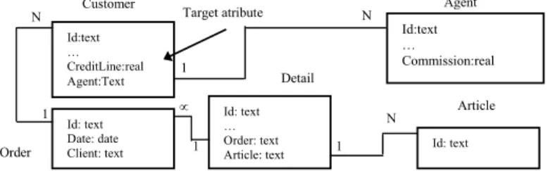
![Fig. 4. Example of (a) refinement (G S ) by adding the a condition on a node not directly connected to the target node, (b) the corresponding complementary refinement, proposed in [11], that does not satisfy the mutual exclusion and (c) correct compleme](https://thumb-eu.123doks.com/thumbv2/5dokinfo/19321138.0/32.892.208.685.352.645/example-refinement-condition-connected-corresponding-complementary-refinement-exclusion.webp)
Inductive Databases of Polynomial Equations
1 Inductive Databases
Various types of patterns have been considered in data mining, including frequent item sets, episodes, datalog queries, and graphs. While many different types of patterns have been considered in data mining, constraints have mainly been considered when mining frequent patterns, usually frequent item sets and association rules.
2 The pattern domain of polynomial equations
- The language of polynomial equations
- Syntactic Constraints
- Evaluation Primitives
- Inductive queries in the domain of equations
The estimation primitives for equations calculate various measures of the degree of fit of the equation to a given data set/table. The second term in the MDL heuristic function introduces a penalty for the complexity of the equation.
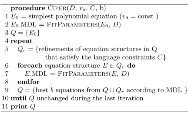
3 A heuristic solver for the domain polynomial equations
Before starting the search process, the Q beam is initialized with the simplest possible polynomial equation of the form vd= const. The value of the constant parameter const is compared to the training data using linear regression and the heuristic MDL function is calculated.
4 Polynomial equations on standard regression datasets
Our approach outperforms linear regression and regression trees and is comparable to model trees. It is interesting to compare the complexity of the equations found by our approach with that of model trees.
5 Using constraints in modeling chemical reactions
The complexity of model trees can be measured as the number of parameters/constants in them, including thresholds in internal nodes and coefficients in leaf linear regressions. The rate of reaction affects the rate of change of all (input and output) compounds involved in the equations.
6 Towards inductive databases for QSAR
The pattern domain of molecular fragments
Cyprus then successfully reconstructs the equations for the entire network, i.e. for each of the 7 system variables, for each of the two beam sizes. Providing Ciperonly with trace behavior and no constraints fails to correctly reconstruct the equations for ˙x1 (beam 128) and ˙x2 (for both beams).
Combining molecular fragments and equations in an inductive database for QSAR
Here one can use the subpolynomial constraints in the equation pattern domain to query equations containing a specific molecular fragment: the fragment in question must be a subpolynomial of the RHS of the equation sought. This is because such comparisons have the same precision/degree of fit as the comparison with a linear degree of the fragment and higher complexity.
Experiments on the biodegradability dataset
Kramer and De Raedt [9] used the two-class version of biodegradability data to mine for interesting features. For the latter two, the comparison was made for both continuous (regression) and discrete (classification via regression) versions of the data set.
7 Summary
CYPER performs much better than J48 for the two-class version and the same for the four-class version.
8 Discussion
In the framework of inductive databases (IDBs), different types of patterns within different so-called pattern domains have been considered [2]. Furthermore, different types of patterns in the same IDB will have to be used for practical applications, such as QSAR (and other applications in bioinformatics).
9 Further work
We believe that both global models (like equations) and local patterns (like molecular fragments) should be considered in IDBs. To our knowledge, global models in the form of equations have not been considered in IDBs so far (although they are routinely used in practical applications, such as QSAR), nor have combinations of local patterns and global models.
Towards Optimizing Conjunctive Inductive Queries
1 Introduction
At this point, the question arises whether we can further exploit the analogy with concept learning to obtain strategies that will minimize the cost of evaluating the patterns. The key contribution of this paper is that we introduce an algorithm for computing the set of solutionsTh(Q,D,L) to a conjunctive inductive query that aims to reduce the cost of evaluating patterns w.t.f.
2 Conjunctive Inductive Queries
We are interested in computing solution sets Th(Q,D,L) for boolean queries Q, which are constructed from monotonic and anti-monotonic pattern predicates. We assume that there are cost functions ca and cm associated with the anti-monotonic and monotonic subqueries Qa and Qm.
3 Solution Methods
- Partial version space trees
- An Algorithmic Framework
- Towards An Optimal Strategy
- Calculating the Counter-Values
If negative, the label is propagated to the leaves by recursively following the incoming suffix links. That is, does it spread to the leaves (following the children- . and incoming suffixes) and does it to the root.

4 Experimental Results
The first thing to note is that in Fig. c) the number of evaluations of Qm is constant for VST. This is more likely to happen in the leaves for smallmax, so in these cases it saves a lot of evaluation of the anti monotonic predicate.

5 Related Work and Conclusions
SIGMOD'96 Workshop on Re- Search Issues on Data Mining and Knowledge Discovery, Montreal, Canada, June 1996. Level search and the limits of theories in knowledge discovery, Data Mining and Knowledge Discovery, vol.
What You Store Is What You Get (extended abstract)
We provide three approaches for obtaining information about the support of element arrays of size less than k. The second approach estimates the support of the itemset by computing it against a pruned database.
2 Preliminaries
This is done by discarding transactions from the database that do not contribute to supporting a frequentk item set and by discarding entries from all transactions that no longer exist in a frequentk item set supported by that transaction. While the frequencies of frequent item sets of greater or equal size can be easily retrieved from such a truncated database, this is less obvious for smaller item sets.
3 Trimming the database
Horizontal Trimming
Vertical Trimming
Combined Trimming
4 Taking care of the smaller itemsets
A naive lossless approach
In addition, the total size of the original database is shown, as well as the total size of all frequent item sets. Note that for this dataset with the minimum support threshold applied, the original database itself is already orders of magnitude smaller than the combined size of all frequent item sets.

A naive lossy approach
A less lossy less naive approach
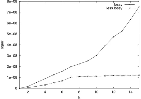
3. The squared error fora= 1 andb= 0 compared to the squared error for the optimal foraandb values for the BMS-Webview-1 database with σ= 36. 4. The ratio of the squared error fora= 1 andb= 0 and the error in square for the optimal foraandb values for the BMS-Webview-1 database with σ= 36.
5 Conclusions and future work
This method is illustrated in Figure 3, where we show the squared error for a= 1 andb= 0 compared to the squared error for optimal values for a and b for the BMS-Webview-1 database with σ = 36. In Figure 4 we compare also the loss approach with the less-loss approach by showing the ratio of the squared error fora= 1 andb= 0 and the squared error for optimal values foraandb.
Acknowledgements
In Proceedings of the 1995 ACM SIGMOD International Conference on Management of Data, deel 24(2) van SIGMOD Record, pagina's 175-186. Srikant, redacteuren, Proceedings of the Seventh ACM SIGKDD International Conference on Knowledge Discovery and Data Mining, pagina's 401–406.
An Algebra for Inductive Query Evaluation
This class is - to the best of the authors' belief - the most expressive class of queries considered so far. On the theoretical side, he has shown that version spaces are closed under intersection, but not under union.
2 Boolean Inductive Queries
The subset of patterns in L that satisfy the predicate Q, composed of monotonic or anti-monotonic predicates using a combination of the 3 logical operators conjunction (∧), negation (¬) and disjunction (∨), is a generalized version space , denoted by T h( Q,D,L). A queryQ has dimension (with respect to the pattern languageL) if the maximum dimension of any solution set Th(Q,D,L) of Q is (where the maximum is taken with all possible data sets Then with the fixed languageL).
3 Operations on Solution Spaces
However, as our general method will show, the dimension of T h(Q2, D,LΣ) is at most two, so it can be represented as the union of two version spaces. Then the dimension of X is equal to the maximum k for which there exists in L an alternating chain of length k (or a k-chain too short) for X.
4 Query Plans and Algebraic Operations
Answering Interactive Queries using Incremental Update Techniques
So we can find out the answer to VS(Q1) by simply performing a filtering operation on VS(Q0). In this case, we can use the incremental update algorithm [14, 15] with adjustments to efficiently compute VS(Q1) using the cached results of VS(Q0).
5 Generalized Version Space Trees
Algorithm TreeMerge
The combination algorithm is presented in the pseudocode in Algorithm 1 as an abstract Boolean operation. When the operation is "and", the flags are combined by conjunction during the merge (interpreted as "false" while ⊕ is treated as "true") and therefore the TreeMerge algorithm will compute the intersection of the represented GVSes.
6 Preliminary Experiments
The Databases
For example, when = ∧ and a certain branch in T1 is empty, there is no need to look for a corresponding branch in T2.
The Queries
In the Unix command database, this question translates to “Which sequences of Unix commands are commonly used by experienced programmers with a length of at least 3 or by computer scientists with a length of at least 2, and are also commonly used by the other two groups users?”. Which amino acid sequences are common in function category 'cat30' with a length of at least 3 or in function category 'cat40' with a length of at least 2, and at the same time common under the function category 'cat2'.
Results
To verify this, we performed experiments on two databases with values for D1, D2, and QA as shown in Table 2. Memory Footprint Not only do we save time but also use memory more efficiently if we use the Q strategy instead of Q for find the set of samples in question.
7 Conclusions
In: Proceedings of The Eight ACM SIGKDD International Conference on Knowledge Discovery and Data Mining, Edmonton, Alberta, Canada (2002). In: Proceedings of the Fifth International Conference on Database Systems for Advanced Applications, Melbourne, Australia.
Finding All Occurring Sets of Interest
Analogous to the set of frequent sets, the set of occurring interesting sets is denoted by . Condensed representations for frequent strings can be tailored to the occurring strings of interest.
2 Mining Closed Occurring Sets of Interest
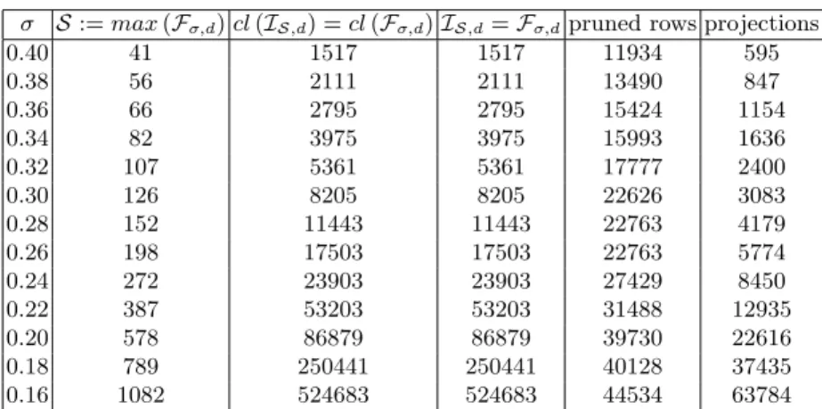
The Intersect-Incremental algorithm finds all closed sets of interest and their frequencies in tidO(nm(|IS,d|+|S|)). The number of sets iS \ IS,d remains zero and they can be removed from the collection IS,d in timeO(|I|).
3 Simplified Databases
The solution found by the heuristic is at least as good as projecting the database onto each set of inS separately.
4 Conclusions
Bouli¸caut, J.F., Bykowski, A., Rigotti, C.: Free sets: a condensed Boolean data representation for approximating frequency queries. In Popa, L., ed.: Proceedings of the Twenty-first ACM Symposium SIGACT-SIGMOD-SIGART on Principles of Database Systems, ACM.
Mining concepts from large SAGE gene expression matrices
Recently, association rule mining has been studied as a complementarity approach for the identification of a priori genes of interest [2]. In Section 2, we define the RNApattern domain and thus an inductive database approach for the analysis of gene expression data.
2 The RNA pattern domain
Mining the frequent sets of genes is specified as the computation of {X∈ LA| Cminfreq(X,r) satisfied}. Mining the closed set of genes is specified as the computation of {X ∈ LA | CCluk(X,r) satisfied}.
3 Inductive query evaluation
Indeed, it is easy to derive the entire collection of frequent gene sets from {X ∈ LA | Cminfreq(X,r)∧ CClose(X,r) satisfied}. In other words, we compute the collection of closed sets of genes as {h(X,r)∈ LA| Cfree(X,r) satisfied}.
4 Applications to SAGE data
The impact of the discretization on the validity/interest of the extracted regularities must be investigated in each context. In all cases for the larger matrices, extraction becomes possible by operating on the transposed matrix.
5 Conclusion
It comes from the combination of an efficient algorithm to compute the closed sets from the free sets and the use of the Galois connectivity properties. Francois Rioult is supported by the IRM department of Caen CHU, comit´e de la Manche de la Ligue contre le Cancer and Conseil R´egional de Basse-Normandie.
Generalized Version Space Trees
Note that generalized version space trees can in principle be used for many different purposes, but our focus here is their use as a condensed representation to speed up typical frequent substructure data mining queries. The use of condensed representations such as generalized version space trees is intended to enable fast access to information about already encountered patterns in main memory at the expense of some memory overhead.
2 Frequent Free Tree Mining
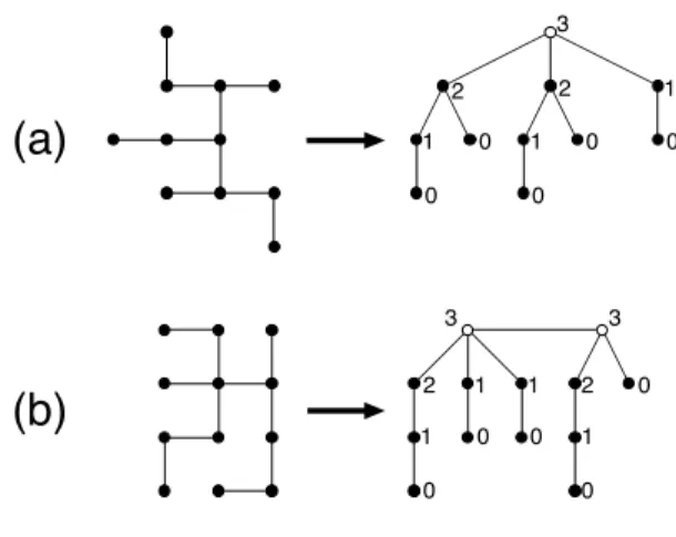
The structural completion of the tree1 with respect to2 is the recursive application of the structural completion for nodes to the nodes often1. The root of the smaller of the two subtrees is used as the root of the entire tree.
3 Generalized Version Space Trees
NCI DTP Anti-Cancer Screening Data
After the global version space tree was calculated, all 100 queries were executed in just 0.2 seconds. That means using the generalized version space tree as a cache structure reduced the total processing time from 24984 seconds to 399 seconds, a time savings of more than 98%.
NCI DTP Anti-HIV Screening Data
It is clear that generalized version space trees are an efficient way to augment similar common substructure queries in databases. However, it is not clear how the spatial requirements of generalized space trees affect its performance.