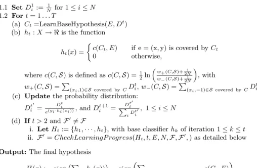
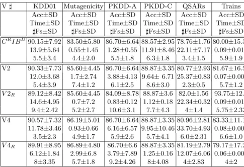
In Section 3, we give a detailed summary of the work done on unit cost active feature selection originally reported in [9] and [8]. At each iterative call t of the base learner, the base hypothesis h t is learned about E based on the current distribution D t .
The learning progress is monitored in terms of the development of the average margins of the training examples. Boosting is known to be particularly effective in increasing the margins of training examples [20, 7].
A Simple Relational Classifier
1 Motivation
While the reported results on the relational classifiers (PRMs, RPTs, and RBCs) have been compared with basic non-relational learners (e.g., the naive Bayes classifier or C4.5 [26]), a simple relational classifier is an equally important, and perhaps a more appropriate point of comparison. Here we analyze the Relational Neighbor (RN) [25] classifier as such a simple classifier that only uses class labels from known related instances and does not learn.
2 A Relational Neighbor Classifier
We then propose a probabilistic version of RN and show that it unexpectedly does not add value in the cases described in this paper, although it may do so in other domains. The iterative relational-neighbor (RN∗) classifier iteratively classifies entities using the RN classifier in its inner loop.
3 Case Studies
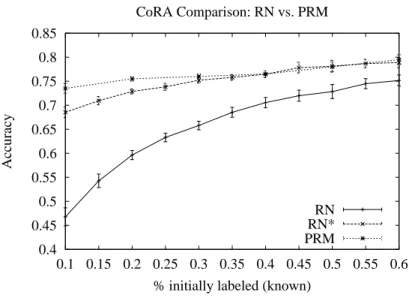
CoRA
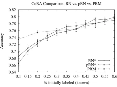
Using the same methodology reported in the PRM study, we ranged the proportion of papers whose class is initially known from 10% to 60%. We will only report on the RN ∗ classifier in the following two studies because of its clear superiority.
IMDb
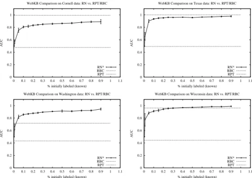
Second, in all cases, although less so in the Cornell data set, RN* was competitive with RPT, even seeing only 5% of the data. In this case, looking at only 5% of the data gave very close performance in 3 out of 4 data sets.
RBC RPT
4 The Probabilistic Relational Neighbor Classifier
Due to the fuzzy nature of the propagation, there is no guarantee of convergence, although in all our test cases, the probabilities appear to be converging. In virtually all tests, when only a small fraction (≤ 30%) of the data was initially labeled, RN ∗ performed better than pRN ∗ , although they often performed similarly when we labeled > 75% of the data.
5 pRN on Synthetic Data
From these results, it is clear that pRN* is able to use very little information (eg, one negative and only one good guy - 0.1% good) to virtually completely characterize the remaining negatives. Even when the bad guys are unknown, pRN ∗ is still able to perform very well.
6 Final Remarks
Acknowledgments
Furthermore, 5% of the good guys need to be labeled before it can perform comparably to pRN. The views and conclusions contained herein are those of the authors and should not be interpreted as necessarily representing the official policies or endorsements, whether expressed or implied, of the Defense Advanced Research Projects Agency (DARPA), the Air Force Research Laboratory, or the U.S. .
This work is sponsored by the Defense Advanced Research Projects Agency (DARPA) and the Air Force Research Laboratory, Air Force Command, USAF, under agreement number F. Technical Report 02-55, Department of Computer Science, University of Massachusetts Amherst, nil Report 02-55, Dept. in Computer Science, University of Massachusetts Amherst, 2002.
Collective Classification with
Relational Dependency Networks
1 Introduction
We show preliminary results showing that collective inference with RDN provides improved performance compared to non-collective inference which we call “individual inference”. We also show that collectively applied RDNs can perform close to the theoretical ceiling reached if all neighbor labels are known with perfect accuracy. These results are very promising, indicating the potential utility of further exploration of collective inference with RDN.
2 Classification Models of Relational Data
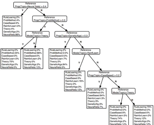
In this article, we present Relational Dependency Networks (RDNs), an undirected graph model for relational data. As a result, learned RPTs are a relatively compact and parsimonious representation of conditional probability distributions in relational data.
3 Relational Dependency Networks
Dependency Networks
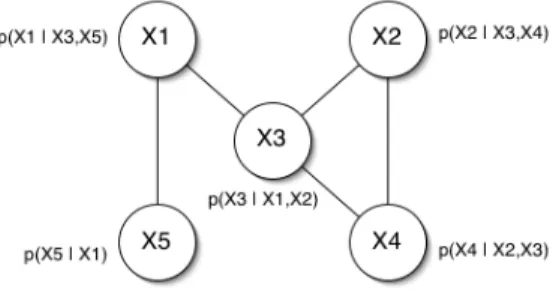
The undirected edges of the graph connect each node x i to each of its parents (the nodes in pa i. Each node is conditionally independent of the other nodes in the graph given its parents.
Learning. As with any graphical model, there are two components to learning a DN
Relational Dependency Networks
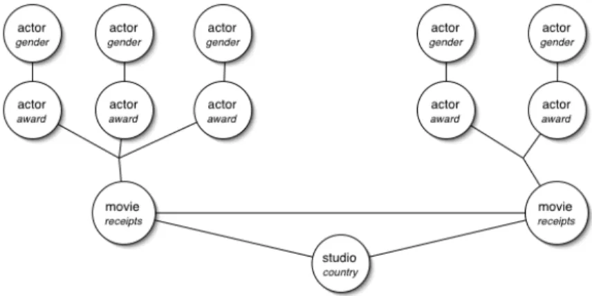
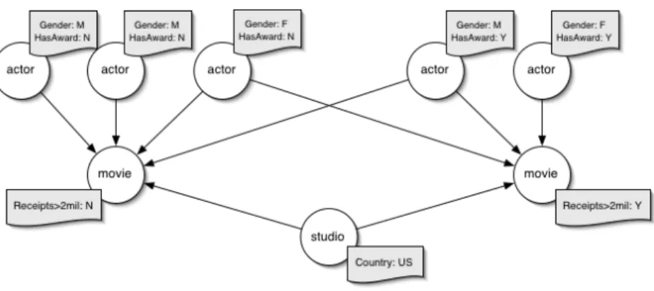
Given a set of objects and the relationships between them, an RDN defines a complete joint probability distribution over the values of the objects' attributes. For each objective variable, the RPT model is used to return a probability distribution given the actual attribute values in the rest of the graph.
4 Experiments
Tasks
Nine attributes were supplied to the models, including country of study, actor's year of birth, and the class label of related movies two links away. Twelve attributes were available for the models, including journal affiliation, paper location, and the subject of articles one link away (references) and two links away (via authors).
Results and Discussion
In addition, the performance of the RDN models is superior to both the RPT-indiv models (RPT learned without labels) and the RPT standard models (RPT learned with labels and tested with a standard labeling for the class values of related instances). If we can conclude from the learning curves that the Gibbs chain had converged, why did the RDN model not perform as well as the RPT ceiling model on Cora.
5 Conclusions and Future Work
The Gibbs chain can mix slowly, making it unlikely that the process will jump to a distant part of the label space. The views and conclusions contained herein are those of the authors and should not be construed to necessarily represent the official policies or endorsements, expressed or implied, of DARPA, AFRL, or the US.
Structural Logistic Regression for Link Analysis
1 Introduction
This is both impractical and incorrect - the size of the resulting table is prohibitive, and the notion of an object corresponding to an observation is lost, being represented by multiple rows. We propose the use of Structural Logistic Regression to link prediction and argue that the properties of the method and the task are a good match.
2 Methodology
We use data from CiteSeer (a.k.a. ResearchIndex), an online digital library of computer science papers [22] ( http://citeseer.org/.
Search
Relational Feature GenerationStatistical Model Selection
Control Module Learning Process
Relational Database Engine
Feature Generation
Refinement graphs are directed acyclic graphs that specify the search space of the first-order logic queries. Using aggregate operators in feature generation makes trimming the search space more involved.
3 Tasks and Data
The latter is easier and should be the subject of future improvements. .. search down refinement graphs allows for a number of optimizations, e.g. i) the results of queries (before applying the aggregations) at a parent node can be reused at the child nodes; this should certainly be weighed against the space required to store the views, and ii) a node whose query results are empty for each observation should not be further refined, as its refinements will also be empty. Density is the percentage of existing citations out of the total number of possibilities, (# Docs)_ Dataset # Docs # Links Density (`a\bc_.
4 Results
We change the ratio of the number of negative examples to the number of positive ones used in testing. Precision recall curves for the “artificial intelligence” dataset with different class priors. is the ratio of the number of negatives to the number of positive examples used in testing.
5 Related Work and Discussion
While in the first case "upgrading" can also be seen as a form of "propositionalization", the second emphasizes that the model selection criteria of the original propositional algorithm do not participate in the construction of properties. Being a domain-wide joint probabilistic model, PRMs can provide answers to a large number of questions, including class labels, latent groups, changing beliefs based on new observations.
6 Conclusions and Future Work
Ðñ0ðGPAïeïePT_4ø(ikK.\ñedlmSQø3i\aedñpd(jNdfe]$MOlkdø(dPAòð\KTør÷ ZTfePBOS\a$÷RSOP*ikdaejïlkSïd.\NdT9lmSïd. d(frKzïødñ_ÕKNSR]6_`PTfød.imlmïgd(frKAiÓñ<ïøî\KNS#SOdø3dñøñgKAfg]pñéPN_`d'iklmïødfgKNiÓñ`ZNdSOd(frKîïïñ`ZNdSOd(frK
BettyJoyce
YpîOd2MOfgdalÓø(KAïdñÇMGdø(lACQø(KAïlkPNS ©
ALEPH BOUNDED mFOIL
S8\_5ðGd(f5PAò*ø3iÓK.\ñÇdñlmï5ø3PTS\ñÇïf;\øზïgda pKNñÕô8AüÚiÓKAfgZNd(f[LKAimïgîOP.OZTîùK2ï*ზñø](Çðñø](Çðø; ø3ï Eda2ò¯PNfÿ *U*e ÐñÍM\f EPETZNfrKA_ PTS .ûEj lÓaEdS\ø3d5ûüRïEfrKNø3ïElkPNS2KASQaÛJlkSO÷.
Efficient Multi-relational Classification by Tuple ID Propagation
1 Introduction
In a database for multi-relational classification, there is one target relation R t , whose tuples are called target tuples. Until now, there is no accurate, efficient and scalable approach for multi-relational classification.
2 Related Works
It uses a sequential covering algorithm that is similar to FOIL, which iteratively builds rules and removes the positive sets of targets covered by each rule. It then constructs a new dataset which contains all positive and negative target tuples satisfying r', along with the corresponding non-target tuples.
Card card-id
At each step, every possible predicate is evaluated and the best one is added to the current rule. After calculating the foil gain of each of these predicates, the best predicate is added to the current rule.
Client client-id
FOIL is inefficient because it has to evaluate too many predicates in the whole procedure, and evaluating each predicate is time-consuming due to the new data set. Therefore, FOIL is not scalable according to the number of relations and the number of attributes in the databases.
3 Tuple ID Propagation
Account
Loan
Basic Definitions
In the example above, a tuple in Loan can only be associated with one tuple in Account. In fact, it can be associated with more than one tuple in other relationships such as Order and Customer (see figure 1).
Search for Predicates by Joins
For a predicate in account relation, such as "Account(A, ?, monthly, ?)", we need to define what is meant by "a target tuple satisfies a rule containing this predicate". We say that a tuple t in the Loan relation satisfies r if and only if a tuple in the Account relation that can be connected to t has value "monthly" on the frequency attribute.
Loan ∞ Account
Tuple ID Propagation
One way to solve this problem is to run the join once and calculate the foil gain of all predicates.
Loan loan-id
Please note that we cannot only calculate the foil gain from the class labels of each tuple in account relations (see Figure 3). For each tuple t in R 2 , there is a set of IDs representing the tuples in the target relation that can be joined to t (using the join path specified in the current rule).
4 Implementation
Data Representation
For example, "Loan(L, A) specifies that we should merge the Account relation with the Loan relation (in our case, propagating the Tulp IDs of the Loan relation into the Account relation). For example, "Account(A, ?, monthly, ?)" specifies that tuples must have the value "monthly" for the frequency attribute in the account relation.
Learning Algorithm
In a predicate pair, the first predicate specifies how we can pass IDs to the relation, and the second predicate specifies the constraint of that relation. Loan(L, A Account(A, ?, monthly, ?))" specifies that we propagate tuple IDs from the Loan relation to the Account relation, and in the Account relation the frequency attribute must have the value "monthly".
We define a predicate pair as the combination of a predicate of the first type p 1 and a predicate of the second type p 2.
5 Experimental Results
We modified the data set a bit by shrinking the Trans relation, which is extremely large, and removing some positive target tuples in the Loan relation to make the number of positive and negative target tuples more balanced.
6 Conclusions
Â_`k i sqfhე~egik¢oq}gkh_kh_ji oqeYfheg|ზმfhpzsvuJჃgfhaji khkhu}Ypr_jჃ!fhe!prვk n¢fheg|ma`k iprprftÃNaji¯Ä.
ÛT59@D=