Fourier Transform 1:

(1)

Fourier Transform 1:

Digital Signal and Image Processing Fourier Theory

Prof. David Marshall

School of Computer Science & Informatics

(2)

Fourier Transform

Moving into the Frequency Domain

The Frequency domain can be obtained through the transformation, via Fourier Transform (FT), from

one (Temporal (Time) or Spatial) domain to the other

Frequency Domain

We do not think in terms of signal or pixel intensities but

rather underlying sinusoidal waveforms of varying frequency,

amplitude and phase.

(3)

Applications of Fourier Transform

Numerous Applications including:

Essential tool for Engineers, Physicists, Mathematicians and Computer Scientists

Fundamental tool for Digital Signal Processing and Image Processing

Many types of Frequency Analysis:

Filtering Noise Removal Signal/Image Analysis

Simple implementation of Convolution Audio and Image Effects Processing.

Signal/Image Restoration — e.g.

Deblurring

Signal/Image Compression —- MPEG (Audio and Video), JPEG use related techniques.

Many more . . . .

3 / 66

(4)

Introducing Frequency Space

1D Audio Example

Lets consider a 1D (e.g. Audio) example to see what the different domains mean:

Consider a complicated sound such as the a chord played on a piano or a guitar.

We can describe this sound in two related ways:

Temporal Domain : Sample the amplitude of the sound many times a second, which gives an approximation to the sound as a function of time.

Frequency Domain : Analyse the sound in terms of the pitches of the notes, or frequencies, which make the sound up, recording the amplitude of each frequency.

Fundamental Frequencies D[ : 554.40Hz

F : 698.48Hz A[ : 830.64Hz C: 1046.56Hz plus harmonics/partial frequencies ....

(5)

Back to Basics

An 8 Hz Sine Wave

A signal that consists of a sinusoidal wave at 8 Hz.

8 Hz means that wave is completing 8 cycles in 1 second

The frequency of that wave is 8 Hz.

From the frequency domain we can see that the composition of our signal is

one peak occurring with a frequency of 8 Hz — there is only one sine wave here.

with a magnitude/fraction of 1.0 i.e. it is the whole signal.

5 / 66

(6)

2D Image Example

What do Frequencies in an Image Mean?

Now images are no more complex really:

Brightness along a line can be recorded as a set of values measured at equally spaced distances apart,

Or equivalently, at a set of spatial frequency values.

Each of these frequency values is a frequency component.

An image is a 2D array of pixel measurements.

We form a 2D grid of spatial frequencies.

A given frequency component now specifies what contribution

is made by data which is changing with specified x and y

direction spatial frequencies.

(7)

Frequency components of an image

What do Frequencies in an Image Mean? (Cont.)

Large values at high frequency components then the data is changing rapidly on a short distance scale.

e.g. a page of text

However, Noise contributes (very) High Frequencies also Large low frequency components then the large scale features of the picture are more important.

e.g. a single fairly simple object which occupies most of the image.

7 / 66

(8)

Visualising Frequency Domain Transforms

Sinusoidal Decomposition

Any digital signal (function) can be decomposed into purely sinusoidal components

Sine waves of different size/shape — varying amplitude, frequency and phase.

When added back together they reconstitute the original signal.

The Fourier transform is the tool that performs such an operation.

(9)

Summing Sine Waves. Example: to give a Square(ish) Wave

Digital signals are composite signals made up of many sinusoidal frequencies

A 200Hz digital signal (square(ish) wave) may be a composed of 200, 600, 1000, etc. sinusoidal signals which sum to give:

9 / 66

(10)

Summary so far

So What Does All This Mean?

Transforming a signal into the frequency domain allows us To see what sine waves make up our underlying signal E.g.

One part sinusoidal wave at 50 Hz and Second part sinusoidal wave at 200 Hz.

Etc.

More complex signals will give more complex decompositions

but the idea is exactly the same.

(11)

How is this Useful then?

Basic Idea of Filtering in Frequency Space

Filtering now involves attenuating or removing certain frequencies — easily performed:

Low pass filter —

Ignore high frequency noise components — make zero or a very low value.

Only store lower frequency components High Pass Filter — opposite of above

Bandpass Filter — only allow frequencies in a certain range.

11 / 66

(12)

Visualising the Frequency Domain

Think Graphic Equaliser

An easy way to visualise what is happening is to think of a graphic equaliser on a stereo system (or some software audio players, e.g.

iTunes).

(13)

So are we ready for the Fourier Transform?

We have all the Tools....

This lecture, so far, (hopefully) set the context for Frequency decomposition.

Past Maths Lectures:

Odd/Even Functions: sin(−x) = − sin(x), cos(−x) = cos(x) Complex Numbers: Phasor Form re

ⁱ^φ

= r (cos φ + i sin φ) Calculus Integration: R

e

^kx

dx =

^e_k^kx

Digital Signal Processing:

Basic Waveform Theory. Sine Wave y = A.sin(2π.n.F

w

/F

s

)

where: A = amplitude, F

w

= wave frequency, F

s

= sample frequency, n is the sample index.

Relationship between Amplitude, Frequency and Phase:

Cosine is a Sine wave 90

^◦

out of phase Impulse Responses

DSP + Image Proc.: Filters and other processing, Convolution

13 / 66

(14)

(15)

Fourier Theory

Introducing The Fourier Transform

The tool which converts a spatial or temporal (real space) description of audio/image data, for example, into one in terms of its frequency components is called the Fourier transform

The new version is usually referred to as the Fourier space description of the data.

We then essentially process the data:

E.g. for filtering basically this means attenuating or setting certain frequencies to zero

We then need to convert data back (or invert) to real audio/imagery to use in our applications.

The corresponding inverse transformation which turns a Fourier space description back into a real space one is called the inverse Fourier transform.

15 / 66

(16)

1D Fourier Transform

1D Case (e.g. Audio Signal)

Considering a continuous function f (x ) of a single variable x representing distance (or time).

The Fourier transform of that function is denoted F (u), where u represents spatial (or temporal) frequency is defined by:

F(u) = Z

∞

−∞

f (x )e

^−2πixu

dx.

Note: In general F(u) will be a complex quantity even though the original data is purely real.

The meaning of this is that not only is the magnitude of each frequency present important, but that its phase relationship is too.

Recall Phasors from Complex Number Lectures.

e

^−2πixu

above is a Phasor.

(17)

Inverse Fourier Transform

Inverse 1D Fourier Transform

The inverse Fourier transform for regenerating f (x) from F (u) is given by

f (x) = Z ∞

−∞

F (u)e ^2πixu du,

which is rather similar to the (forward) Fourier transform except that the exponential term has the opposite sign.

It is not negative

17 / 66

(18)

Fourier Transform Example

Fourier Transform of a Top Hat Function

Let’s see how we compute a Fourier Transform: consider a particular function f (x) defined as

f (x) =

1 if |x| ≤ 1 0 otherwise,

1 1

(19)

The Sinc Function (1)

We derive the Sinc function

So its Fourier transform is:

F(u) = Z_∞

−∞

f(x)e^−2πixudx

= Z₁

−1

1×e^−2πixudx

= −1

2πiu(e^2πiu−e^−2πiu)

Now (refer toComplex NumbersLectures/Maths Formula SheetHandout)

sinθ = e^iθ−e^−iθ 2i ,So:

F(u) = sin2πu πu .

In this case,F(u)ispurely real, which is a consequence of the original data beingsymmetricinxand−x.

f(x)is anevenfunction.

A graph ofF(u)is shown overleaf.

This function is often referred to as theSinc function. 19 / 66

(20)

The Sinc Function Graph

The Sinc Function

The Fourier transform of a top hat function, the Sinc function:

−6 −4 −2 0 2 4 6

−0.5 0 0.5 1 1.5 2

u sin(2 π u)/(π u)

(21)

The 2D Fourier Transform

2D Case (e.g. Image data)

If f (x, y) is a function, for example intensities in an image, its Fourier transform is given by

F (u , v) = Z ∞

−∞

Z ∞

−∞

f (x, y)e −2πi(xu+yv)

dx dy ,

and the inverse transform, as might be expected, is

f (x, y) = Z ∞

−∞

Z ∞

−∞

F (u, v)e ^2πi(xu+yv) du dv .

21 / 66

(22)

The Discrete Fourier Transform

But All Our Audio and Image data are Digitised!!

Thus, we need a discrete formulation of the Fourier transform:

Assumes regularly spaced data values, and

Returns the value of the Fourier transform for a set of values in frequency space which are equally spaced.

This is done quite naturally by replacing the integral by a

summation, to give the discrete Fourier transform or DFT for

short.

(23)

1D Discrete Fourier transform (DFT)

1D Case:

In 1D it is convenient now to assume that x goes up in steps of 1, and that there are N samples, at values of x from 0 to N − 1.

So the DFT takes the form

F (u) = 1 N

N−1

X

x=0

f (x)e

^−2πixu/N

,

while the inverse DFT is

f (x) =

N−1

X

u=0

F (u)e

^2πixu/N

.

NOTE: Minor changes from the continuous case are a factor of 1/N in the exponential terms, and also the factor 1/N in front of the forward transform which does not appear in the inverse transform.

23 / 66

(24)

2D Discrete Fourier transform

2D Case

The 2D DFT works is similar.

So for an N × M grid in x and y we have

F (u, v) = 1 NM

N−1

X

x=0 M−1

X

y=0

f (x, y)e −2πi(xu/N+yv/M) ,

and

f (x, y ) =

N−1

X

u=0 M−1

X

v=0

F (u, v)e 2πi(xu/N+yv/M) .

(25)

Balancing the 2D DFT

Most Images are Square

Often N = M , and it is then it is more convenient to redefine F (u , v) by multiplying it by a factor of N, so that the forward and inverse transforms are more symmetric:

F (u , v) = 1 N

N−1

X

x=0 N−1

X

y=0

f (x, y)e −2πi(xu+yv)/N , and

f (x, y) = 1 N

N−1

X

u=0 N−1

X

v=0

F (u, v)e 2πi(xu+yv)/N .

25 / 66

(26)

Fourier Transforms in MATLAB

fft() and fft2()

MATLAB provides functions for 1D and 2D Discrete Fourier Transforms (DFT):

fft(X) is the 1D discrete Fourier transform (DFT) of vector X. For matrices, the FFT operation is applied to each column — NOT a 2D DFT transform.

fft2(X) returns the 2D Fourier transform of matrix X. If X is a vector, the result will have the same orientation.

fftn(X) returns the N-D discrete Fourier transform of the N-D array X.

Inverse DFT ifft(), ifft2(), ifftn() perform the inverse DFT.

See appropriate MATLAB help/doc pages for full details.

Plenty of examples to Follow.

→ Transforms → Fourier Transform

(27)

Visualising the Fourier Transform

Visualising the Fourier Transform Having computed a DFT it might be useful to visualise its result:

It’s useful to visualise the Fourier Transform

Standard tools

Easily plotted in MATLAB

0 2 4 6 8 10 12 14 16

−1 0 1

n →

a)

Cosine signal x(n)

0 2 4 6 8 10 12 14 16

0 0.5 1

k →

b)

Magnitude spectrum |X(k)|

0 0.5 1 1.5 2 2.5 3 3.5

x 10⁴ 0

0.5 1

f in Hz →

c)

Magnitude spectrum |X(f)|

27 / 66

(28)

The Magnitude Spectrum of Fourier Transform

Recall that the Fourier Transform of our real audio/image data is always complex

Phasors: This is how we encode the phase of the underlying signal’s Fourier Components.

How can we visualise a complex data array?

Back to Complex Numbers:

Magnitude spectrum Compute the absolute value of the complex data:

|F (k)| = q

F

_R²

(k) + F

_I²

(k) for k = 0, 1, . . . , N − 1

where F

R

(k) is the real part and F

I

(k) is the imaginary part of the N sampled Fourier Transform, F(k).

Recall MATLAB: Sp = abs(fft(X,N))/N;

(Normalised form)

(29)

The Phase Spectrum of Fourier Transform

The Phase Spectrum Phase Spectrum

The Fourier Transform also represent phase, the phase spectrum is given by:

ϕ = arctan F _I (k )

F _R (k ) for k = 0, 1, . . . , N − 1

Recall MATLAB: phi = angle(fft(X,N))

29 / 66

(30)

Relating a Sample Point to a Frequency Point

When plotting graphs of Fourier Spectra and doing other DFT processing we may wish to plot the x-axis in Hz (Frequency) rather than sample point number k = 0, 1, . . . , N − 1

There is a simple relation between the two:

The sample points go in steps k = 0, 1, . . . , N − 1

For a given sample point k the frequency relating to this is given by:

f _k = k f s

N

where f s is the sampling frequency and N the number of samples.

Thus we have equidistant frequency steps of ^f _N

^s

ranging

from 0 Hz to ^N−1 _N f s Hz

(31)

MATLAB Fourier Frequency Spectra Example

fourierspectraeg.m

N=16;

x=cos(2*pi*2*(0:1:N-1)/N)'; figure(1)

subplot(3,1,1);

stem(0:N-1,x,'.');

axis([-0.2N-1.2 1.2]);

legend('Cosine signal x(n)');

ylabel('a)');

xlabel('n \rightarrow');

X=abs(fft(x,N))/N;

subplot(3,1,2);stem(0:N-1,X,'.');

axis([-0.2N-0.1 1.1]);

legend('Magnitude spectrum |X(k)|');

ylabel('b)');

xlabel('k \rightarrow') N=1024;

x=cos(2*pi*(2*1024/16)*(0:1:N-1)/N)';

FS=40000;

f=((0:N-1)/N)*FS;

X =abs(fft(x,N))/N;

subplot(3,1,3);plot(f,X);

axis([-0.2*44100/16max(f)-0.1 1.1]);

legend('Magnitude spectrum |X(f)|');

ylabel('c)');

xlabel('f in Hz \rightarrow') figure(2)

subplot(3,1,1);

plot(f,20*log10(X./(0.5)));

axis([-0.2*44100/16max(f)...

-45 20]);

legend('Magnitude spectrum |X(f)| ...

in dB');

ylabel('|X(f)| in dB \rightarrow');

xlabel('f in Hz \rightarrow')

31 / 66

(32)

MATLAB Fourier Frequency Spectra Example Output

fourierspectraeg.m produces the following:

0 2 4 6 8 10 12 14 16

−1 0 1

n →

a)

Cosine signal x(n)

0 2 4 6 8 10 12 14 16

0 0.5 1

k →

b)

Magnitude spectrum |X(k)|

0 0.5 1 1.5 2 2.5 3 3.5

x 10⁴ 0

0.5 1

f in Hz →

c)

Magnitude spectrum |X(f)|

(33)

Magnitude Spectrum in dB

Note: It is common to plot both spectra magnitude (also frequency ranges not show here) on a dB/log scale:

(Last Plot in fourierspectraeg.m)

0 0.5 1 1.5 2 2.5 3 3.5

x 10⁴

−40

−20 0 20

f in Hz →

|X(f)| in dB → Magnitude spectrum |X(f)| in dB

33 / 66

(34)

Time-Frequency Representation: Spectrogram

Spectrogram

It is often useful to look at the frequency distribution over a short-time:

Split signal into N segments

Do a windowed Fourier Transform — Short-Time Fourier Transform (STFT)

Window needed to reduce leakage effect of doing a shorter sample SFFT.

Apply a Blackman, Hamming or Hanning Window MATLAB function does the job: Spectrogram — see help spectrogram

MATLAB spectrogram Example

spectrogrameg.m

load( ' handel ' ) [N M] = size(y);

figure(1)

spectrogram(y,512,20,1024,Fs);

Produces the following:

35 / 66

(36)

Aphex Twin Spectrogram

Aphex Twin famously ¹ embedded images in the spectrogram of a few tracks on his Windowlicker EP. His face on Track 2 “Formula”

or “Equation” (Full title:

^∆Mi−1=−αPN n=1D_i[n][P

σ∈C[i]F_ji[n−1] +Fext_i[n−1]]

!!:

1

See here for web link to other examples of embedded image Spectrograms

(37)

Matlab Code to show the Aphex Twin Spectrogram

Previous slide use the free and excellent Sonic Visualiser We of course know how to display the image in MATLAB:

37 / 66

(38)

Matlab Code to show the Aphex Twin Spectrogram

Aphex Spectrogram.m

aphex = audioread('FormulaSnippet.wav');

mono = (aphex(:,1) + aphex(:,2))/2;

spectrogram(mono,1024,120,2048,'power','yaxis');

set(gca, ' YScale ' , ' log ' );

colormap( ' winter ' );

xlabel('Time')

ylabel( ' Frequency (Log Scale) ' )

Note: we change the display of the spectrogram to a log scale, which looks better.

Audio clip here: FormulaSnippet.wav

(39)

So what does my face sound like?

Let’s embed my face in spectrogram:

It sounds like this:

0 5 10 15

x 10⁴

−1

−0.5 0 0.5 1

Daphex

39 / 66

(40)

Image to Sound Conversion

Daphex.m

figure(1);

imshow(imread('Dave_Frame0001.jpg'));

dave_im2snd = im2sound('Dave_Frame0001','jpg',44100,40,6000,0.00002,10);

sound(dave_im2snd,44100);

figure(2);

spectrogram(dave_im2snd,1024,120,2048,'power','yaxis');

set(gca,'YScale','log');

colormap('winter');

shg;

Image used here: Dave Frame0001.jpg

(41)

Image to Sound Conversion ²

im2sound.m (Usage)

function[final_sound] = im2sound(filename, ext, f_sample, f_low,...

f_high, amp_mod, sample_t)

%INPUTS:

%'filename'- Name of the image to be encoded (not including extension

%ext'- Extension of the image (not including "." at the beginning).

%'f_sample'- Sampling frequency (Hz)

%'f_low'- Lowest frequency (Hz) (e.g. 40)

%'f_high'- Highest frequency (Hz) (e.g. 6000)

%'amp_mod'- Multiplication factor for the amplitude. Decrease until

%image is clear. Too high and the waveform clips. Too low and the image

%is very dark (e.g. 0.00002)

%'sample_t'- Duration of the sample in seconds. Longer samples have

%better quality (e.g. 10)

%OUTPUTS:

%'final_sound'- the final sound containing the image. This is

%automatically saved to a .wav file with the original image filename

2

Original Code from MATLAB Central

41 / 66

(42)

Image to Sound Conversion

im2sound.m (Code)

function[final_sound] = im2sound(filename, ext, f_sample, f_low,...

f_high, amp_mod, sample_t) ...

%INITIALISING VARIABLES:

%The waveform at each time point. This is reset at the beginning of each

%time point temp_sound =0;

%The final waveform final_sound =0;

%MAIN BODY

%Loading the sample image and calculating the image size raw_im = imread(strcat(filename,'.',ext));

size_raw_im =size(raw_im);

%Making a frequency table for the height of the image. Each row of the

%image is assigned a particular frequency from the corresponding row of

%this table. The frequencies are linearly distributed between the highest and

%lowest user-definied frequencies. "f_step" is the increment between each

%adjacent frequency

f_step = (f_high-f_low)/size_raw_im(1,1);

f_table = (f_high:-f_step:f_low);

(43)

Image to Sound Conversion

im2sound.m (Code)

%The final sound will dwell on each column of the image for a specific

%time. This time is defined by "t_start" and "t_end". It depends on how

%long the user determined the sound-clip should be and how wide (how many

%columns) the image is.

t_step = (sample_t/size_raw_im(1,2));

%Initial values for the start and end times. These will be increased at

%the end of each loop iteration (when the script moves onto the next column

%of the image).

t_start =0;

t_end = t_step;

%The loop which generates the sound file. At each iteration it generates a

%segment of the final sound file, which is temporarily saved to

%"temp_sound". This segment is built up of frequencies from that

%particular column of the image.

for j=1:size_raw_im(1,2)

%Initialising the variable (the sound for each frequency (row) is added

%to the existing sound) temp_sound =0;

%Setting the time in matrix format t = t_start:1/f_sample:(t_end);

43 / 66

(44)

Image to Sound Conversion

im2sound.m (Code)

%For each iteration of this loop, the script goes down the current

%column of the image and generates a waveform of the frequency

%specified in "f_table". The amplitude of the waveform is determined

%by the pixel intensity. This generated waveform is added to all the

%previously generated waveforms in that particular column for i= size_raw_im(1,1):-1:1

temp_sound = temp_sound+sin(2*pi*t*f_table(i))*...

double(raw_im(i,j))*amp_mod;

end

%At the end of each column the segment of sound generated is added to

%the end of the existing sound file ("final_sound").

final_sound =cat(2,final_sound,temp_sound);

%The temporary sound is cleared ready for the start of the next column clear temp_sound

%Moving to the next time frame t_start = t_start+t_step;

t_end = t_end+t_step;

end

%This saves "final_sound" to the'.wav'file of the same name as the input

%file

wavwrite(final_sound, f_sample, strcat(filename,'.wav'));

(45)

Properties of Fourier Transforms

Here are just a few of the other properties of Fourier transforms which are useful when reasoning, or computing, with Fourier transforms:

Linear Operator Shifting

Scaling Rotation

Zeroth component

Convolution Theorem (see next section applications)

45 / 66

(46)

Fourier Transform: Linear Operator

The Fourier transform is a linear operator. This means that Theorem

If f (x) and g (x) are two functions with Fourier transforms F(u)

and G (u), then the Fourier transform of af (x) + bg (x) where a

and b are constants is simply aF(u) + bG (u).

(47)

Linear Operator Simple Example

Image 1 Image 2

Image 3

47 / 66

(48)

Linear Operator Simple Example

Image 1 + Image 2 Spectra

50 100 150 200 250

50

100

150

200

250

imft3 Spectra

50 100 150 200 250

50

100

150

200

250

Inverse FT of imft1 + imft2

(49)

Linear Operator Simple Example

Fourier Transform Linear Operator Demo: FFT Linear.m

% Create a white box on a black background image M=256; N =256;

image1 =zeros(M,N);

box =ones(64,64);

%box at centre

image1(97:160,97:160) = box;

figure(1) imshow(image1) title('Image 1');

% Create another white box on a black background image M=256; N =256;

image2 =zeros(M,N);

box =ones(32,32);

%box at centre

image2(37:68,37:68) = box;

49 / 66

(50)

Linear Operator Simple Example

Fourier Transform Linear Operator Demo: FFT Linear.m

% Make composite image image3 = image1+image2;

% Compute Fourier Transforms.

imft1 = fft2(double(image1));

figure(4)

imagesc(abs(imft1+imft2)) title('Image 1 + Image 2 Spectra');

figure(5) imagesc(abs(imft3)) title('imft3 Spectra');

figure(6)

imagesc(abs(imft1+imft2-imft3))

title('Difference (Image 1 + Image 2) - imft3 Spectra');

figure(7)

imshow(ifft2(imft1+imft2));

title('Inverse FT of imft1 + imft2');

(51)

Fourier Transform: Shifting

Shifting the real space data through a fixed distance has the effect that

Theorem

If f (x) is a function with Fourier transform F (u), then the Fourier transform of f (x − x 0 ) is given by e ^−2πix

⁰

^u F (u).

Note: that the exponential term here has unit magnitude for all values of u.

Thus, the magnitude of the resulting Fourier transform is left unchanged, although the relative sizes of the real and imaginary parts are altered.

51 / 66

(52)

Shifting Operator Simple Example

FT of Image 1 (imft1)

50 100 150 200 250

50

100

150

200

250

FT of Image 2 (imft2)

50 100 150 200 250

50

100

150

200

250

(53)

Shifting Operator Simple Example

Inverse FT of imft3 Image 2

Both Images are the same.

FT of imft3 (imft1 shifted in Fourier Space

50 100 150 200 250

50

100

150

200

250

Residual of IFT of imft3 and image2

53 / 66

(54)

Shifting Operator Simple Example

Fourier Transform Shifting Operator Demo: FFT Shift.m

% Define Initial box x0 =97;

y0 =97;

xwidth =64;

ywidth =64;

image1 =zeros(M,N);

box =ones(xwidth,ywidth);

%box at centre

image1(x0:x0+xwidth-1,y0:y0+ywidth-1) = box;

% Define shift dx=40;

dy=0;

% Shift Image 1 image2 =zeros(M,N);

image2(x0+dx:x0+dx+xwidth-1,y0+dy:y0+dy+ywidth-1) = box;

(55)

Shifting Operator Simple Example

Fourier Transform Shifting Operator Demo: FFT Shift.m

% Compute Fourier Transfoms.

figure(3)

imagesc(abs(fftshift(imft1)));

title('FT of Image 1 (imft1)');

figure(4)

title('FT of Image 2 (imft2)');

% Define shift in frequency domain [yF,xF] =meshgrid(-M/2:M/2-1,-N/2:N/2-1);

% Perform the shift

imft3=imft1.*exp(-1i*2*pi.*(xF*dx+yF*dy)/256);

figure(5)

title('FT of imft3 (imft1 shifted in Fourier Space');

figure(6)

imshow(ifft2(imft3));

title('Inverse FT of imft3');

figure(7)

imshow(ifft2(imft3)-image2);

title('Residual of IFT of imft3 and image2'); 55 / 66

(56)

Fourier Transform: Scaling

If we scale the spacing of the real space data in distance, we have that

Theorem

If f (x) is a function with Fourier transform F (u), then the Fourier transform of f (ax ) where a is a real constant is given by _|a| ¹ F ( ^u _a ).

In other words:

if we spread out the data in real space, the data is compressed into more compact region of Fourier space.

This is intuitive — if we double the spacing of a grid pattern, its spatial frequency is halved.

Note that the magnitude of the Fourier representation is

also affected.

(57)

Scaling Operator Simple Example

Fourier Transform of Image 1 (imft1)

50 100 150 200 250

50

100

150

200

250

50 100 150 200 250

50

100

150

200

250

57 / 66

(58)

Scaling Operator Simple Example

Fourier Transform Scaling Operator Demo: FFT Scale.m

% Define Initial box xwidth =40;

ywidth =40;

x0 = M/2 -xwidth/2;

y0 = N/2 -ywidth/2;

image1 =zeros(M,N);

%box at centre

% Define scale scalex =0.5;

scaley =0.5;

% Image 2 = Scaled Image 1 image2 =zeros(M,N);

[px,qx] =rat(scalex);

[py,qy] =rat(scaley);

(59)

Scaling Operator Simple Example

Fourier Transform Scaling Operator Demo: FFT Scale.m

in_image2 = resample(resample(double(image1),px,qx)',py,qy)'; xrange = int16(M/2-M*scalex/2:M/2+M*scalex/2-1);

yrange = int16(N/2-N*scaley/2:N/2+N*scaley/2-1);

image2(xrange,yrange)= in_image2;

figure(1) imshow(image1);

title('Image 1');

figure(2) imshow(image2);

title('Image 2');

figure(3)

imagesc(abs(fftshift(imft1)))

title('Fourier Transform of Image 1 (imft1)');

figure(4)

imagesc(abs(fftshift(imft2)))

title('Fourier Transform of Image 2 (imft2)');

59 / 66

(60)

2D Fourier Transform: Rotation

One useful property in two dimensions is that:

if we rotate the real space data, its Fourier transform is rotated by the same angle, or more exactly

Theorem

If f (x, y) is a function with Fourier transform F (u, v ), on expressing these functions in terms of polar coordinates r, θ, ρ, φ where x = r cos θ, y = r sin θ, u = ρ cos φ, v = ρ sin φ so that f (x, y) and F (u, v ) become f (r, θ) and F (ρ, φ) respectively, the Fourier transform of f (r , θ + ω) where ω is a constant is given by F (ρ, φ + ω).

Basically this means the two-dimensional Fourier transform

is an intrinsic property of the data which is independent of

our choice of axis directions.

(61)

Rotation Operator Simple Example

50 100 150 200 250

50

100

150

200

250

50 100 150 200 250

50

100

150

200

250

61 / 66

(62)

Rotation Operator Simple Example

Fourier Transform Rotate Operator Demo: FFT Rotate.m

% Define Initial box xwidth =64;

ywidth =32;

image1 =zeros(M,N);

x0 = M/2 -xwidth/2;

y0 = N/2 -ywidth/2;

%box at centre

% Define Rotation in degrees rot =45;

image2 = imrotate(image1, rot,'bilinear','crop');

figure(1); imshow(image1);

title('Image 1');

figure(2); imshow(image2);

title('Image 2');

imft1 = fftshift(fft2(double(image1)));

imft2 = fftshift(fft2(double(image2)));

figure(3); imagesc(abs(imft1)) title('Fourier Transform of

Image 1 (imft1)');

figure(4); imagesc(abs(imft2)) title('Fourier Transform of I

mage 2 (imft2)');

(63)

Fourier Transform: Zeroth Component

A final property is that the zeroth component of the Fourier space representation is just the average data value (apart from a factor of 1/N, in two dimensions – assuming balanced FT)).

This is illustrated below for the two-dimensional DFT case:

F (u, v) = 1 N

N−1

X

x=0 N−1

X

y=0

f (x, y )e ^−2πi ^(xu+yv)/N , (1) so

F (0, 0) = 1 N

N−1

X

x=0 N−1

X

y =0

f (x, y) = Nf (x , y). (2)

63 / 66

(64)

Simple Zeroth Component Example

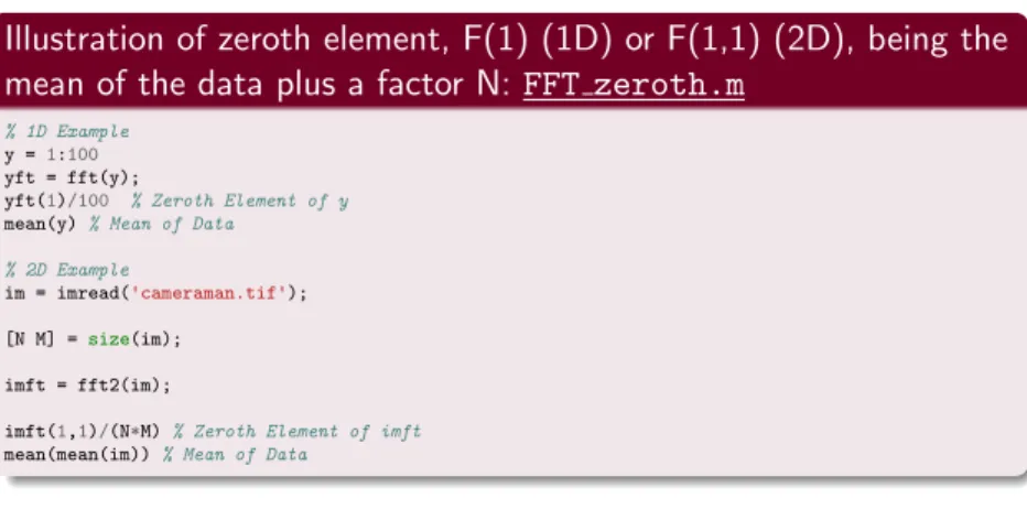
Illustration of zeroth element, F(1) (1D) or F(1,1) (2D), being the mean of the data plus a factor N: FFT zeroth.m

% 1D Example y =1:100 yft = fft(y);

yft(1)/100 % Zeroth Element of y mean(y)% Mean of Data

% 2D Example

im = imread('cameraman.tif');

[N M] =size(im);

imft = fft2(im);

imft(1,1)/(N*M)% Zeroth Element of imft mean(mean(im))% Mean of Data

FT is not balanced in MATLAB

(65)

Corollary: Shifting the Fourier Transform, fftshift()

Centring the Frequency of a Fourier Transform

Most computations of FFT represent the frequency from 0 — N − 1 samples (similarly in 2D, 3D etc.) with corresponding frequencies ordered accordingly — the 0 frequency is not really the centre.

We frequently like to visualise the FFT as the centre of the spectrum.

In 1D (Audio/Vector): swaps the left and right halves of the vector

Similarly in 2D (Image/Matrix) we swap the first quadrant with the third and the second quadrant with the fourth:

This is possible due the invariant shift property of the Fourier Transform.

65 / 66

(66)