At time 1 of the procedure, importance sampling (IS) is used to approximate pθ.x1|y1/ using an importance densityeqθ.x1|y1/. This procedure provides us at time T with an approximation of the joint posterior density pθ.x1:T|y1:T/given by. In the following we will refer to MCMC algorithms targeting the np.θ,x1:T|y1:T/ distribution which rely on sampling exactly from gapθ.x1:T|y1:T/ as 'idealized' algorithms.
We first introduce in Section 2.4.1 the particle-independent Metropolis–Hastings (PIMH) update, an exact approximation to a standard independent Metropolis–Hastings (IMH) targeting pθ.x1:T|y1:T/, which uses SMC approximations of pθ. x1:T|y1:T/as proposition. Our discussion of SMC methods suggests exploring the idea of using the SMC approximation of pθ.x1:T|y1:T/as a propositional density, i.e. Assume for the moment that sampling from the conditional density θ.x1:T|y1:T/for every θ∈Θ is feasible and recall the standard decomposition p.θ,x1:T|y1:T/=p.θ|y1:T / pθ.x1:T|y1:T/.
Again, sampling from pθ.x1:T|y1:T/is typically impossible and we explore the possibility of using a particle approach to this algorithm. It is clear that the naive particle approximation to the Gibbs sampler where sampling from pθ.x1:T|y1:T/ is replaced by sampling from an SMC approximation ˆpθ.x1:T|y1:T/ not p.θ, x1:T does not allow |y1:T/as invariant density.
Applications
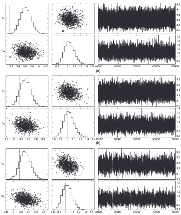
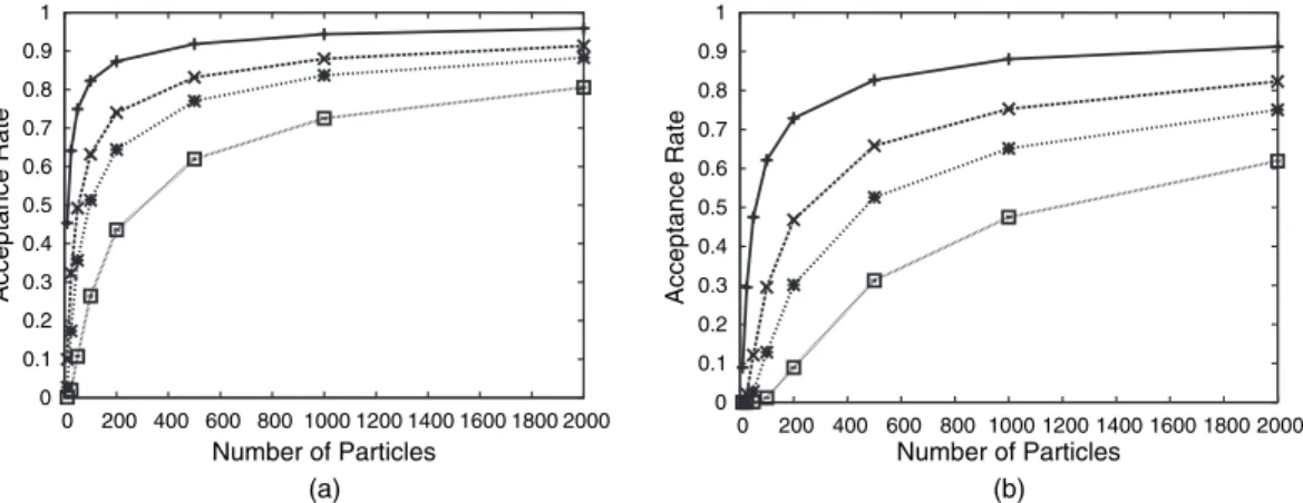
Determining a reasonable trade-off between the average acceptance rate of the PIMH update and the number of particles appears to be difficult. However, this algorithm tends to get stuck in a local mode of the multimodal posterior distribution. This occurred in most runs when using the initializations from the previous forX1:T and results in an overestimation of the true value of σV.
Let Δ denote the length of time between two periods of interest; then the increments of the integrated volatility correspond. Carrying out reasoning in this context is difficult, since the transient precursor of the latent process Xn:=.σ2.nΔ/,z.λnΔ// cannot be expressed analytically. In Creal (2008), an SMC method is proposed for sampling from pθ.x1:T|y1:T/, which uses a truncated prior as the template density, assuming that all hyperparameters of the θmodel are known.
We used a normal random walk MH proposal to update the parameters together, the covariance of the proposal is the estimated covariance of the target distribution which was obtained in a preliminary run. We also use a MH proposal with a normal random walk, the covariance of the proposal is the estimated covariance of the target distribution which was obtained in a prior run.
A generic framework for particle Markov chain Monte Carlo methods
To sample from π.x1:P/ we can propose a PIMH sampler, which is an IMH sampler using an SMC approximation ˆπN.dx1:P/orπ.x1:P/ as a proposal distribution. In light of the discussion in Section 4.1, the SMC algorithm generates the set of random variables X¯1. Moreover, by formulating the PIMH sampler as a disguised IMH targeting algorithmπ˜we can use standard results regarding the convergence properties of the IMH sampler to characterize those of the PIMH sampler. a) the PIMH sampler generates a series {X1:P.i/} whose marginal distributions satisfy {LN{X1:P.i/∈ ·}}.
We use an SMC algorithm to sample approximately πθ.x1:P/ and calculate the approximate normalizing constant γ.θ/. Our main result is the following theorem, which is proven in Appendix B. a) the PMMH update is an MH update defined on the extended space Θ×X with target density. However, sampling from πθ.x1:P/ is obviously impossible in most interesting situations, but is dictated by the structure and properties of π˜N.θ,k,x¯1,.
We have the following result. a) the PG update defines a transition kernel on the extended spaceΘ×X of invariant density. N}the set of proposed weighted particles at iterationi (i.e. before deciding whether to accept this population or not) and ˆγN{θÅ.i/}the associated normalizing constant estimate.
Discussion and extensions
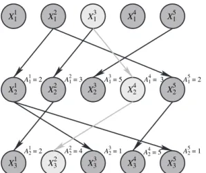
For this, we want to minimize the number of times the conditioned path particle is resampled in each iteration. Consider timing and assume that the conditioned path consists of the first particle at both times nandn+1 (in the notation of the article Bn=1 and Bn+1=1). More specifically, in the notation of the article, a flexible resampling scheme works as follows.
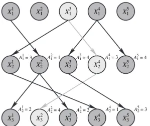
A key ingredient is the elucidation of the probability model underlying a sequential Monte Carlo (SMC) algorithm and the genealogical tree structures that it generates. Another advantage of the particle Hastings–Metropolis algorithm is that it is trivial to parallelize. Our comments on adaptive sequential Monte Carlo (SMC) methods concern particle Metropolis–Hastings (PMH) sampling, which has acceptance probability given in equation (13) in the paper for proposed mode .θÅ,XÅ1:T/, depending on the estimate .
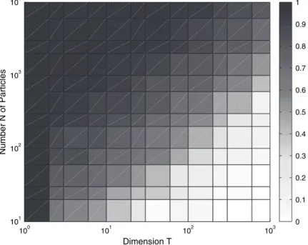
Particle Markov chain Monte Carlo (PMCMC) performance depends on the trade-off between degeneracy of the filter,N, and design of the SMC mutation kernel. In the conclusion, the authors state that the performance of particle MCMC algorithms will depend on the variance of the SMC estimates of the normalizing constants. For example, how does the dimension of the state vector (or state space) affect the algorithm.
It arrives (practically) under the assumption that the state space of the hidden Markov state process is compact. This extends the utility of particle Markov chain Monte Carlo methods to a very broad class of models where likelihood estimation is difficult (or even difficult), but forward simulation is possible. The particle marginal Metropolis–Hastings (PMMH) algorithm is perhaps the simplest of the presented algorithms, relying only on the unbiasedness of the marginal likelihood estimator.
Zp.y,z|θ/dz=p.y|θ/: .55/ An interesting feature of the sequential Monte Carlo class of methods is that the choice of auxiliary variables is flexible. This is essentially an example of the method described here as particle marginal Metropolis–Hastings (PMMH) sampling. As a result of the resampling, the weakest hypotheses die, and the resulting particle collection often gives a good representation of the posterior distribution (Toivanen and Lampinen, 2009a, b).
Dependence on N of the performance of the PMCMC algorithms considered in the paper has two different forms, at first apparently unrelated. Some results illustrating the effect of the non-performance of the MCMC algorithm can be found in Andrieu and Roberts (2009). In this situation, the extended target distribution of the paper takes the particularly simple form (we omit subscript 1 to simplify the notation).
In light of the discussion above, the SMC conditional update provides the ability to target π.xa:b|x1:P\a:b/for 1abP.