Symbolic Model Checking for Probabilistic Timed Automata

Symbolic Model Checking for Probabilistic Timed Automata

Marta Kwiatkowska¹, Gethin Norman¹ and Jeremy Sproston²

1 School of Computer Science, University of Birmingham, Edgbaston, Birmingham B15 2TT, United Kingdom

2 Dipartimento di Informatica, Universit`a di Torino, 10149 Torino, Italy

October 24, 2003

Abstract

Probabilistic timed automata are an extension of timed automata with discrete probability distributions, and can be used to model timed randomized protocols or fault-tolerant sys- tems. We present symbolic model checking algorithms for probabilistic timed automata to verify qualitative properties, corresponding to satisfaction with probability 0 or 1, as well as quantitative properties, corresponding to satisfaction with arbitrary probability. The algorithms operate on zones, that is, sets of valuations of the probabilistic timed automa- ton’s clocks, and therefore avoid an explicit construction of the state space. Our method considers only those system behaviours which guarantee the divergence of time with prob- ability 1. The paper completes the symbolic framework for the verification of probabilistic timed automata against full PTCTL. We formulate new algorithms that can return the minimal probability with which a probabilistic timed automaton satisfies a property, thus extending a previously published result concerning the maximum probability.

1 Introduction

Systems exhibiting bothtimed andprobabilistic characteristics are widespread, in application contexts as diverse as home entertainment, medical equipment and business infrastructures.

For example, timing constraints are often vital to the correctness of embedded digital technol- ogy, whereas probability exhibits itself commonly in the form of statistical estimates regarding the environment in which a system is embedded. Similarly, protocol designers often exploit the combination of time and probability to design correct, efficient protocols, such as the IEEE1394 FireWire root contention protocol. The diffusion of such systems has led to meth- ods for obtaining formal correctness guarantees, for instance, adaptations of model checking [CGP99]. Symbolic model checking refers to model-checking techniques in which implicit rep- resentations – such as BDDs in the finite-state case [BCM⁺90] – are used to represent both the transition relation of the system model and the state sets that are computed during the execution of the model-checking algorithm.

In this paper, we consider the modelling formalism ofprobabilistic timed automata[KNSS02], an extension of timed automata [AD94, HNSY94] with discrete probability distributions.

∗Supported in part by the EPSRC grant GR/N22960, FORWARD and MIUR-FIRB Perf.

Technical Report CSR-03-10, School of Computer Science, University of Birmingham, October 2003.

Probabilistic timed automata have been shown as being suitable for the description of timed, randomized protocols, such as the aforementioned FireWire protocol [KNS03], the backoff strategy of the IEEE802.11 WLAN protocol [KNS02], and the link-local address selection protocol of the IPv4 standard [KNPS03]. As a requirement specification language for proba- bilistic timed automata we consider PTCTL (Probabilistic Timed Computation Tree Logic).

The logic PTCTL combines the probabilistic threshold operator of the probabilistic tem- poral logic PCTL [HJ94] with the timing constraints of the timed temporal logic TCTL [ACD93, HNSY94], in order to express properties such as ‘with probability 0.99 or greater, the system reaches a leader-elected state within 1 second’. Model checking of probabilistic timed automata against PTCTL was shown to be decidable in [KNSS02] via an adaptation of the classical region-graph construction [AD94, ACD93].

Unfortunately, the region-graph construction (and the integer-time semantics employed in [KNS03, KNS02, KNPS03]) can result in huge state spaces if the maximal constant used in the description of the automaton is large. Instead, the practical success ofsymbolic,zone- based techniques for non-probabilistic timed automata [BDL⁺01, DOTY96], suggests that a similar symbolic approach may also be employed for the verification of probabilistic timed automata. This hypothesis was answered affirmatively in [KNS01] for a subset of PTCTL with thresholds on maximal reachability probabilities. In this paper, we extend that result to arbitrary PTCTL formulae. In particular, a zone-based method for verification of properties which refer to the minimum probability of satisfaction is presented for the first time.

The technical contribution of this paper is the introduction of zone-based algorithms, both for the verification of qualitative PTCTL formulae, which refer to probabilistic thresholds 0 and 1 only, and quantitative PTCTL formulae, which feature thresholds on arbitrary proba- bilities. Note that the qualitative algorithms do not refer to exact transition probabilities, and therefore avoid potentially expensive computation of probabilities during the model-checking process.

We first consider the subset of PTCTL which requires the computation of maximal prob- abilities. For qualitative formulae, we show that model checking can be performed using ana- logues from the verification of finite-state probabilistic systems [dA97], while, in the quantita- tive case, we show that the previously published zone-based approach for calculating maximal probabilities [KNS01] can be employed. The quantitative algorithm works by constructing a finite-state system which has sufficient information to compute the maximum probability of interest using well-established finite-state model checking methods [BdA95].

Secondly, we consider algorithms for the subset of PTCTL which requires the computation of minimum reachability probabilities, a task which is more involved than computing maxi- mum probabilities. For example, to compute the minimum probability of reaching a certain state set F, for any state other than those in F, the probabilistic timed automaton could exhibit behaviour in which the amount of time elapsed converges before F is reached, or even in which no time elapses at all. Clearly, such behaviours are pathological, and should be dis- regarded during model checking. We present both qualitative and quantitative algorithms for computing minimum reachability probabilities which consider only time-divergent behaviour, based on the non-probabilistic precedent of [HNSY94]. The algorithms are based on comput- ing maximum probabilities for the dual formula while restricting attention to time-divergent behaviours.

Finally, again following the precedent of [HNSY94], we present an algorithm to check that a probabilistic timed automaton does not contain a state in which it is impossible for time to diverge with probability 1. The presence of such a state constitutes a modelling error, and

would invalidate the correctness of our model checking procedure.

2 Preliminaries

2.1 Distributions and Probabilistic Systems

A (discrete probability)distribution over a finite set Qis a function µ:Q→[0,1] such that P

q∈Qµ(q) = 1. Let support(µ) be the subset of Q such that q ∈ support(µ) if and only if µ(q)>0. For a possibly uncountable setQ⁰, letDist(Q⁰) be the set of distributions over finite subsets ofQ⁰. For anyq∈Q, the point distributionµq denotes the distribution which assigns probability 1 toq.

2.2 Discrete Time Markov Chains

Definition 1 A DTMC is a tuple DTMC= (S,P,L) where:

• S is a finite set of states;

• P:S×S → [0,1]is a transition probability matrix, such that: P

s⁰∈SP(s, s⁰) = 1 for all states s∈S;

• L:S →2^AP is a labelling functionassigning atomic propositions to states.

Each element P(s, s⁰) of the transition probability matrix gives the probability of making a transition from statesto state s⁰. An execution of a DTMC is represented by apathω, that is, a non-empty sequence of statess0s1s2. . . where si ∈S and P(si, si+1) >0 for all i>0.

We denote by ω(i) the ith state of a path ω, |ω| the length of ω and if ω is finite, the last state bylast(ω). We say that a finite pathω_fin of lengthn is aprefixof an infinite pathω if ω_fin(i) = ω(i) for 0 6i 6n. The sets of all finite and infinite paths starting in state s are denotedPath_ful(s) and Path_fin(s), respectively.

In reason about the probabilistic behaviour of the DTMC, we need to determine the probability that certain paths are taken. This is achieved by defining, for each states∈S, a probability measureProbsoverPathful(s). Below, we give an outline of this construction. For further details, see [KSK76]. The probability measure is induced by the transition probability matrix P as follows. First, for any finite path ω_fin ∈ Path_fin(s), we define the probability Ps(ωfin):

P_s(ω_fin)^def=

1 ifn= 0 P(ω_fin(0), ω_fin(1))· · ·P(ω_fin(n−1), ω_fin(n)) otherwise wheren=|ω_fin|. Next, we define the cylinderof a finite pathωfin as:

C(ωfin)^def={ω∈Pathful(s)|ωfin is a prefix of ω},

and let Σ_s be the smallest σ-algebra on Path_ful(s) which contains the cylinders C(ω_fin) for ωfin ∈Pathfin(s)} and setProbs on Σs to be the unique measure such that

Prob_s(C(ω_fin)) =P_s(ω_fin) for allω_fin ∈Path_fin(s).

2.3 Probabilistic Systems

We next recall probabilistic systems which are essentially equivalent to Markov decision pro- cesses [Der70] and probabilistic-nondeterministic systems [BdA95].

Definition 2 A probabilistic system,PS, is a tuple (S,Steps,L) where

• S is a set of states;

• Steps ⊆S×Dist(S) is a probabilistic transition relation;

• L:S →2^AP is a labelling functionassigning atomic propositions to states.

A probabilistic transition s −→^µ s⁰ is made from a state s by nondeterministically selecting a distributionµ ∈Dist(S) such that (s, µ) ∈Steps, and then making a probabilistic choice of target states⁰ according to µ, such thatµ(s⁰)>0.

We consider two ways in which a probabilistic system’s computation may be represented.

A path, representing a particular resolution of both nondeterminism and probability, is a non-empty sequence of transitions:

ω=s0 µ0

−→s1 µ1

−→s2 µ2

−→ · · · .

We use the same notation for paths as presented in Section 2.2, in particular, the set of infinite (respectively, finite) paths starting in the state s are denoted by Path_ful(s) (respectively, Path_fin(s)).

In contrast to a path, an adversaryrepresents a particular resolution of nondeterminism only. Formally, an adversary A is a function mapping every finite pathω_fin to a distribution µ such that (last(ω_fin), µ) ∈ Steps. For any adversary A and state s, we let Path^A_ful(s) (respectively, Path^A_fin(s)) denotes the subset of Path_ful(s) (respectively, Path_fin(s)) which corresponds to A and, using classical techniques [KSK76], we can define the probability measureProb^A_s overPath^A_ful(s).

For a given adversaryA and finite pathω, we define a new adversary A_ω as follows:

Aω(ω⁰)^def=

A(ω−→^µ ω⁰⁰) ifω⁰ is of the formlast(ω)−→^µ ω⁰⁰ A(ω⁰) otherwise.

Whenever possible, the adversary Aω acts essentially as A assuming that the path ω has already taken place.

For a probabilistic systemPS= (S,Steps,L) and states∈S, under a given adversaryA, the behaviour from statescan be described with the infinite-state DTMCDTMC^A= (S^A,P^A) where: S^A=Path_fin(s) and for two finite pathsω_fin, ω⁰_fin ∈S^A:

P^A(ω_fin, ω_fin⁰ ) = (

µ(s⁰) ifω⁰_fin is of the formωfin

A(ωfin)

−−−−→s⁰ and A(ω) =µ 0 otherwise.

There is a one-to-one correspondence between the paths of DTMC^A and the set of paths Path^A_ful(s), and hence using the construction given in Section 2.2 we can define a probability measureProb^A_s overPath^A_ful(s).

For a probabilistic systemPS= (S,Steps,L), states∈S, setF ⊆S of target states, and adversary A∈AdvPS, let:

ProbReach^A(s, F)^def= Prob^A_s{ω∈Path^A_ful(s)| ∃i∈N. ω(i)∈F},

then the maximal reachability probabilitiesof reaching the set of statesF fromsis defined as:

MaxProbReach(s, F)^def= sup

A∈AdvPS

ProbReach^A(s, F). 2.4 Timed Probabilistic Systems

We now introduce timed probabilistic systems, an extension of probabilistic systems and a variant of Segala’s probabilistic timed automata [Seg95].

Definition 3 A timed probabilistic system, TPS, is a tuple (S,Steps,L) where:

• S is a set of states;

• Steps ⊆S×R×Dist(S)is atimed probabilistic transition relation, such that, if(s, t, µ)∈ Steps and t>0, then µis a point distribution;

• L:S →2^AP is a labelling function.

The componentt of a tuple (s, t, µ) is called aduration. As for probabilistic systems, we can introduce paths and adversaries for timed probabilistic systems, except transitions are now labelled by duration-distribution pairs and an adversary maps each finite path to a duration- distribution pair.

We restrict attention totime-divergent adversaries; a common restriction imposed in real- time systems so that unrealisable behaviour (i.e. corresponding to time not advancing beyond a bound) is disregarded during analysis. For any path

ω =s₀−−−→^t0,µ0 s₁−−−→^t1,µ1 s₂−−−→ · · ·^t2,µ2

of a timed probabilistic system, the duration up to the n+1th state of ω, denoted D_ω(n+1), equals Pn

i=0t_i, and we say that a pathω isdivergent if for anyt∈R, there existsj∈Nsuch thatD_ω(j)>t.

Definition 4 An adversary Aof a timed probabilistic system TPSisdivergent if and only if for each states of TPS the probability under Prob^A_s of the divergent paths of Path^A_ful(s) is 1.

Let Adv_TPS be the set of divergent adversaries of TPS.

For motivation on why we considerprobabilistic divergence, as opposed to the stronger notion where an adversary is divergent if and only if all its paths are divergent, see [KNSS02]. A restriction we impose on probabilistic timed systems is that ofnon-zenoness, which stipulates that there does not exist a state from which time cannot diverge, as we consider this situation to be a modelling error.

Definition 5 A probabilistic timed system is non-zenoif and only if there exists a divergent adversary.

3 Probabilistic Timed Automata

In this section we review the definition of probabilistic timed automata [KNSS02], a modelling framework for real-time systems exhibiting both nondeterministic and stochastic behaviour.

The formalism is derived from classical timed automata [AD94, HNSY94] extended with discrete probability distributions over edges.

3.1 Clocks and Zones

Let X be a finite set of variables called clocks which take values from the time domain R (non-negative reals). A point v ∈ R^{|X |} is referred to as a clock valuation. For any clock x∈ X, we use v(x) to denote the projection of v on thex-axis. For any v ∈R^{|X |} and t∈R, we usev+tto denote the clock valuation defined asv(x)+tfor all x∈ X. We usev[X:=0] to denote the clock valuation obtained fromv by resetting all of the clocks in X ⊆ X to 0, and leaving the values of all other clocks unchanged.

The set of zones of X, writtenZones(X), is defined inductively by the syntax:

ζ ::=x6d|c6x|x+c6y+d| ¬ζ|ζ∨ζ

where x, y ∈ X and c, d ∈ N. We only consider canonical zones ensuring equality between their syntactic and semantic (subsets of R^{|X |}) representations. This enables us to use the above syntax interchangeably with set-theoretic operations.

The clock valuationvsatisfiesthe zoneζ, writtenv .ζ, if and only ifζ resolves to true after substituting each clockx ∈ X with the corresponding clock value v(x) from v. We require the following classical operations on zones [HNSY94, Tri98]. For any zonesζ, ζ⁰ ∈Zones(X) and subset of clocksX⊆ X, let:

._ζ⁰ ζ ^def= {v| ∃t>0.(v+t . ζ ∧ ∀t⁰ 6t.(v+t⁰. ζ∨ζ⁰))}

[X := 0]ζ ^def= {v|v[X:= 0]. ζ} ζ[X:= 0] ^def= {v[X := 0]|v∈ζ}.

3.2 Syntax and Semantics of Probabilistic Timed Automata

Definition 6 A probabilistic timed automaton is a tuple (L,X,inv,prob,L) where:

• L is a finite set of locations;

• the function inv :L→Zones(X) is theinvariant condition;

• the finite set prob ⊆L×Zones(X)×Dist(2^X×L) is theprobabilistic edge relation;

• L:L→2^AP is a labelling function assigning atomic propositions to locations.

Astate of a probabilistic timed automatonPTAis a pair (l, v)∈L×R^{|X |} such thatv .inv(l).

Informally, the behaviour of a probabilistic timed automaton can be understood as follows.

In any state (l, v), there is a nondeterministic choice of either (1) making adiscrete transition or (2) letting time pass. In case (1), a discrete transition can be made according to any (l, g, p) ∈ prob with source location l which is enabled; that is, zone g is satisfied by the current clock valuationv. Then the probability of moving to the location l⁰ and resetting all

true x63 x>1

x62 di

sr si

x>2

0.9 0.1

x:=0 x:=0

0.95 x:=0

0.05 x:=0

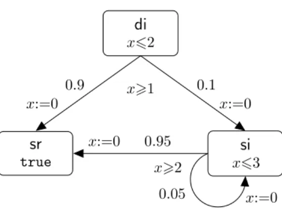
Figure 1: A probabilistic timed automaton modelling a probabilistic protocol.

of the clocks in X to 0 is given by p(X, l⁰). In case (2), the option of letting time pass is available only if the invariant condition inv(l) is satisfied while time elapses.

An edge e of PTA is a tuple of the form (l, g, p, X, l⁰) such that (l, g, p) ∈ prob and p(X, l⁰)>0. Letedgesdenote the set of edges andedges(l, g, p) the set of edges corresponding to (l, g, p)∈prob.

Example. Consider thePTAmodelling a simple probabilistic communication protocol given in Figure 1. The nodes represent the locations: di (sender has data, receiver idle);si (sender sent data, receiver idle); and sr(sender sent data, receiver received). The automaton starts in location diin which data has been received by the sender. After between 1 and 2 time units, the protocol makes a transition either to srwith probability 0.9 (data received), or tosiwith probability 0.1 (data lost). In si after 2 to 3 time units, the protocol will attempt to resend the data, which again can be lost, this time with probability 0.05.

We now give the semantics of probabilistic timed automata defined in terms of timed proba- bilistic systems.

Definition 7 Let PTA= (L,X,inv,prob,L) be a probabilistic timed automaton. Theseman- tics of PTA is defined as the timed probabilistic system TPS_PTA = (S,Steps,L⁰) where:

• S ⊆L×R^{|X |} and(l, v)∈S if and only if v .inv(l);

• ((l, v), t, µ)∈Steps if and only if one of the following conditions holds time transitions: t>0, µ=µ_(l,v+t) and v+t⁰.inv(l) for all 06t⁰6t

discrete transitions: t=0 and there exists(l, g, p)∈prob such that v . g and for any (l⁰, v⁰)∈S:

µ(l⁰, v⁰) = X

X⊆X&

v⁰=v[X:=0]

p(X, l⁰);

• L⁰(l, v) =L(l) for any(l, v)∈S.

We say that PTA is non-zeno if and only ifTPS_PTA is non-zeno.

3.3 Probabilistic Timed Computation Tree Logic (PTCTL)

We now describe the probabilistic timed logic PTCTL which can be used to specify properties of probabilistic timed automata. PTCTL is a combination of two extensions of the tempo- ral logic CTL, the timed logic TCTL [ACD93, HNSY94] and the probabilistic logic PCTL [HJ94]. The logic TCTL employs a set of formula clocks, Z, disjoint from the clocks X of the probabilistic timed automaton. Formula clocks are assigned values by a formula clock valuation E ∈ R^|Z|. The logic TCTL can express timing constraints and includes the reset quantifierz.φ, used to reset the formula clockz so that φis evaluated from a state at which z= 0. PTCTL is obtained by enhancing TCTL with the probabilistic quantifier P_∼λ[·].

Definition 8 The syntax of PTCTLis defined as follows:

φ::=a ζ

¬φ

φ∨φ z.φ

P_∼λ[φ U φ]

where a∈AP, ζ ∈Zones(X ∪ Z), z∈ Z, ∼ ∈ {6, <, >,>} and λ∈[0,1].

In PTCTL we can express properties such as ‘with probability at least 0.95, the system clock x does not exceed 3 before 8 time units elapse’, which is represented as the formula z.P_>0.95[(x63)U (z=8)].

We write v,E to denote the composite clock valuation in R^{|X ∪Z|} obtained from v ∈R^{|X |} and E ∈R^|Z|. Given a state and formula clock valuation pair (l, v),E, zoneζ and durationt, by abuse of notation we let (l, v),E. ζ denote v,E. ζ, and (l, v)+tdenote (l, v+t).

Definition 9 Let TPS= (S,Steps,L⁰) be the timed probabilistic system associated with the probabilistic timed automaton PTA. For any state s ∈ S, formula clock valuation E ∈ R^|Z|

and PTCTL formula θ, the satisfaction relation s,E |=θ is defined inductively as follows:

s,E |=a ⇔ a∈ L⁰(s) s,E |=ζ ⇔ s,E. ζ

s,E |=φ∨ψ ⇔ s,E |=φors,E |=ψ s,E |=¬φ ⇔ s,E 6|=φ

s,E |=z.φ ⇔ s,E[z:= 0]|=φ

s,E |=P_∼λ[φ U ψ] ⇔ p^A_s,E(φU ψ)∼λ for allA∈Adv_TPS

where p^A_s,E(φ U ψ) = Prob^A_s{ω ∈ Path^A_ful(s)|ω,E |= φU ψ} for any A ∈ Adv_TPS, and, for any path ω ∈ Pathful(s), we have that ω,E |= φ U ψ if and only if there exists i ∈ N and t6D_ω(i+1)−D_ω(i) such that

• ω(i)+t,E+D_ω(i)+t|=ψ;

• if t⁰ < t, then ω(i)+t⁰,E+D_ω(i)+t⁰ |=φ∨ψ;

• if j < i and t⁰ 6D_ω(j+1)−D_ω(j), then ω(j)+t⁰,E+D_ω(j)+t⁰ |=φ∨ψ.

In the following sections we will also consider the dual of the sub-formula φU ψ, namely the release formula ¬φV ¬ψ, where for any formulae φ, ψ, path ω and formula clock evaluation E: ω,E |=φV ψ if and only if for alli∈Nand t6D_ω(i+1)−D_ω(i), if

• ω(i)+t⁰,E+D_ω(i)+t⁰ 6|=φ∧ψ for allt⁰ < t and

• ω(j)+t⁰,E+D_ω(j)+t⁰6|=φ∧ψ for all t⁰6D_ω(j+1)−D_ω(j) and j < i,

thenω(i)+t,E+D_ω(i)+t|=ψ.

Furthermore, we use use the abbreviation 2φfor the formula false V φ, that is, ω,E |= 2ψ if and only if ω(i)+t,E+D_ω(i)+t |= ψ for all i ∈ N and t 6 D_ω(i+1)−D_ω(i). In the standard manner, we refer toφ U ψ,φV ψ and 2ψ aspath formulae.

We now present a number of lemmas concerning PTCTL that we will require in the remainder of the paper.

Lemma 10 Let PTA be a timed probabilistic automaton, TPS= (S,Steps,L⁰) be the corre- sponding timed probabilistic system and φ,ψ₁ andψ₂ PTCTLformulae. If s,E |=ψ₁ implies s,E |= ψ₂ for all state and formula clock valuation pairs s,E ∈ S×R^Z, then for any state and formula clock valuation pair s,E ∈S×R^Z:

• s,E |=P_.λ[φ U ψ2]implies s,E |=P_.λ[φ U ψ1],

• s,E |=z.ψ₁ implies s,E |=z.ψ₂.

Proof. The proof follows from the semantics of PTCTL (see Definition 9). ut Lemma 11 LetPTAbe a probabilistic timed automata,PS= (S,Steps,L⁰) be the correspond- ing timed probabilistic system andφandψare PTCTL formulae. Ifs,E |=ψ impliess,E |=φ for all state and formula clock valuation pairs s,E ∈S×R^|Z|, then for any (infinite) pathω of TPSand formula clock valuation E:

ω,E |=φU ψ if and only if ω,E 6|=¬ψ U ¬φ .

Proof. LetPTAbe a probabilistic timed automaton,TPS= (S,Steps,L⁰) be the correspond- ing timed probabilistic system and φ and ψ be PTCTL formulae such thats,E |=ψ implies s,E |=φfor all state and formula clock valuation pairss,E ∈S×R^|Z|. For the ‘if’ direction, consider any infinite path of TPSand formula clock valuation E such thatω,E |=φU ψ. By Definition 9, there exists an i>0 and t6D_ω(i+1)−D_ω(i) such that:

• ω(i)+t,E+D_ω(i)+t|=ψ;

• ift⁰ < t, then ω(i)+t⁰,E+D_ω(i)+t⁰ |=φ∨ψ;

• ifj < i and t⁰6D_ω(j+1)−D_ω(j), then ω(j)+t⁰,E+D_ω(j)+t⁰ |=φ∨ψ.

Therefore, using the fact that s,E |= ψ implies s,E |=φ for all s,E ∈S×R^|Z|, there exists an i>0 andt6D_ω(i+1)−D_ω(i) such that:

• ω(i)+t,E+D_ω(i)+t6|=¬ψ∨ ¬φ;

• ift⁰ < t, then ω(i)+t⁰,E+D_ω(i)+t⁰ 6|=¬φ;

• ifj < i and t⁰6D_ω(j+1)−D_ω(j), then ω(j)+t⁰,E+D_ω(j)+t⁰ 6|=¬φ.

and hence ω,E 6|=¬ψ U ¬φ. Since this was for any pathω ofTPSthe ‘if’ direction holds.

The ‘only if’ direction follows similarly, using the identity ¬¬θ ≡ θ and since, from the hypothesis, s,E |=¬φimplies s,E |=¬ψfor all s,E ∈S×R^|Z|. ut The lemma below use the measure construction for probabilistic systems given in Section 2.3 and recall that, the states of the DTMC corresponding to an adversaryA and statesare the finite paths of A that start in state s. Furthermore, it follows from this construction that a finite path (state in the DTMC) satisfies a formula when the last state of the path satisfies the formula.

Lemma 12 Let PTA be a probabilistic timed automaton and TPS = (S,Steps,L⁰) be the corresponding timed probabilistic system. For any PTCTL formulae φ and ψ, adversary A∈Adv_TPS and state and formula clock valuation pair s,E ∈S×R^|Z|:

p^A_s,E(ψ U (φ∧ψ)∨p^A_>1(2(¬φ∧ψ))) =p^A_s,E(φ V ψ) where for anyω,E ∈Path^A_fin(s)× E^|Z|:

ω,E |=p^A_>1(2(¬φ∧ψ)) if and only if p^A_last^ω_(ω),E(2(¬φ∧ψ)) = 1.

Proof. Consider any probabilistic timed automataPTA with associated timed probabilistic system TPS= (S,Steps,L⁰), adversary A ∈ Adv_TPS and PTCTL formulae φ and ψ. First, for any finite pathω ofPath^A_fin and formula clock valuationE, ifω,E |=p^A_>1(2(¬φ∧ψ)), then ω⁰,E |=2(¬φ∧ψ) for all (infinite) pathsω⁰ ∈Path^A_ful^ω(last(ω)). Therefore, for any finite path ω ofPath^A_fin and formula clock valuation E:

ω,E ∈p^A_>1(2(¬φ∧ψ)) ⇒ ω⁰,E 6|=¬φU ¬ψ for allω⁰ ∈Path^A_ful^ω(last(ω))). (1)

Now by Definition 9, for any (infinite) pathω⁰ ofTPSand formula clock valuation E ∈R^|Z|: ω⁰,E |=¬φU ¬ψ⇔ ω⁰,E |= (¬φ∨ ¬ψ) U ¬ψ

⇔ ω⁰,E |= (¬φ∨ ¬ψ)∧ ¬p^A_>1(2(¬φ∧ψ))

U ¬ψ by (1).

Therefore, by the dualityφU ψ≡ ¬(¬φ V ¬ψ) and the definition ofA_ω (sse Section 2.3), it follows that for any state and formula clock valuation pairs,E ∈S×R^|Z|:

p^A_s,E(φV ψ) = 1−p^A_s,E(((¬φ∨ ¬ψ)∧ ¬p^A_>1(2(¬φ∧ψ))) U ¬ψ)

= 1−p^A_s,E(¬((φ∧ψ)∨p^A_>1(2(¬φ∧ψ)))U ¬ψ) (2) where the last step follows from the following derivation:

((¬φ∨ ¬ψ)∧ ¬p^A_>1(2(¬φ∧ψ))) ≡ (¬(φ∧ψ)∧ ¬p^A_>1(2(¬φ∧ψ)))

≡ ¬((φ∧ψ)∨p^A_>1(2(¬φ∧ψ))).

Finally, since for any finite pathω and formula clock valuationE we have ω,E |=¬ψ implies

ω,E |=¬((φ∧ψ)∨p^A_>1(2(¬φ∧ψ))), applying Lemma 11 to (2) we have that for any state and

formula clock valuation pairs,E ∈S×R^|Z|:

p^A_s,E(φV ψ) = 1−(1−p^A_s,E(ψU (φ∧ψ)∨p^A_>1(2(¬φ∧ψ))))

= p^A_s,E(ψ U (φ∧ψ)∨p^A_>1(2(¬φ∧ψ)))

as required. ut

algorithmPTCTLModelCheck(PTA, θ) output: set of symbolic states [[θ]] such that

[[a]] :={(l,inv(l))|l∈L andl∈ L(a)};

[[ζ]] :={(l,inv(l)∧ζ)|l∈L};

[[¬φ]] :={(l,inv(l)∧ ¬W

(l,ζ)∈[[φ]]ζ)|l∈L};

[[φ∨ψ]] := [[φ]]∨[[ψ]];

[[z.φ]] :={(l,[{z}:=0]ζ)|(l, ζ)∈[[φ]]};

[[P_∼λ[φU ψ]]] :=Until([[φ]],[[ψ]],∼λ);

Figure 2: Symbolic PTCTL model checking algorithm

4 Symbolic PTCTL Model Checking

In this section, we show how a probabilistic timed automaton may be model checked against PTCTL formulae. In order to represent the state sets computed during the model checking process, we use the concept of symbolic state: a symbolic state is a pair (l, ζ) comprising a location and a zone over X ∪Z. The set of state and formula clock valuation pairs corre- sponding to a symbolic state (l, ζ) is {(l, v),E |v,E . ζ}, while the state set corresponding to a set of symbolic states is the union of those corresponding to each individual symbolic state. In the manner standard for model checking, we progress up the parse tree of a PTCTL formula, from the leaves to the root, recursively calling the algorithm PTCTLModelCheck, shown in Figure 2, to compute the set of symbolic states which satisfy each subformula. Han- dling observables and Boolean operations is classical, and we therefore reduce our problem to computing Until([[φ₁]],[[φ₂]],∼λ), which arises when we check probabilistically quantified formula.

Our technique depends on the following, which is a direct consequence of the semantics of PTCTL (Definition 9):

{s,E |s,E |=P_∼λ[φU ψ]}=

{s,E |p^max_s,E (φU ψ)∼λ} if∼∈ {<,6}

{s,E |p^min_s,E (φU ψ)∼λ} if∼∈ {>, >} (3) where for any PTCTL path formulaϕ:

p^max_s,E (ϕ)^def= sup_A∈Adv

TPSp^A_s,E(ϕ) and p^min_s,E (ϕ)^def= infA∈Adv_TPSp^A_s,E(ϕ).

We begin by introducing operations on symbolic states. In Section 4.2, we review algorithms for calculating maximum probabilities, while in Section 4.3 we present new algorithms for calculating minimum probabilities. In each case we include specialised algorithms for qual- itative formulae (λ ∈ {0,1}), as, for such formulae, verification can be performed through only an analysis of the underlying graph [HSP83, Pnu83]. Then in Section 4.4 we show how to ensure that the probabilistic timed automaton is non-zeno and, finally, in Section 4.5, we apply our approach to the example given in Figure 1.

Note that the cases P_>0[·] and P₆₁[·] are trivially satisfied by all states, while the cases P_<0[·] andP_>1[·] are trivially not satisfied by any state, and therefore we omit these cases in our analysis.

algorithmpre0(V) Y:= [[false]]

fore∈edges Y:=Y∨dpre(e,V) end

return Y

algorithmpre1(U,V) Y:= [[false]]

for (l, g, p)∈prob Y0 := [[true]]

Y1 := [[false]]

fore∈edges(l, g, p) Y0:=dpre(e,U)∧Y0

Y1:=dpre(e,V)∨Y1

end

Y:= (Y₀∧Y1)∨Y end

return Y

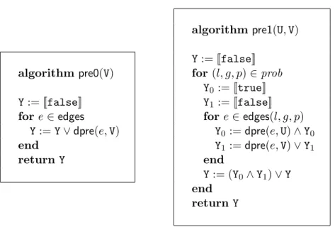
Figure 3: The functionspre0 and pre1 4.1 Operations on Symbolic States

In this section we extend the time predecessor and discrete predecessor functions tpre and dpre of [HNSY94, Tri98] to probabilistic timed automata. For any sets of symbolic states U,V⊆L×Zones(X ∪Z), clock x∈ X ∪ Z and edge (l, g, p, X, l⁰):

x.U ^def= {(l,[{x}:=0]ζ_U^l)|l∈L}

tpre_U(V) ^def= {(l,._ζl

U∧inv(l)(ζ_V^l ∧inv(l))|l∈L}

dpre((l, g, p, X, l⁰),U) ^def= {(l, g∧([X:= 0]ζ_U^l0))}. where ζ_U^l = W

{ζ|(l, ζ) ∈ U}, i.e ζ_U^l is the zone such that v,E. ζ_U^l if and only if (l, v),E ∈ u for some u∈U. Furthermore, we define the conjunction and disjunction of sets of symbolic states as follows:

U∧V^def={(l, ζ_U^l ∧ζ_V^l)|l∈L} and U∨V^def={(l, ζ_U^l ∨ζ_V^l)|l∈L}.

Finally, let [[false]] = ∅and [[true]] = {(l,inv(l))|l∈L}, the sets of symbolic states repre- senting the empty and full state sets respectively.

4.2 Computing Maximum Probabilities

In this section we review the methods for calculating the set of states satisfying a formula of the formP_.λ[φU ψ] which, from (3), reduces to the computation ofp^max_s,E (φU ψ) for all state and formula clock valuation pairss,E. Note that, since we consider only non-zeno automata, when calculating these sets we can ignore the restriction to divergent adversaries. This is similar to verifying the same type of properties against (finite state) probabilistic systems with fairness constraints [BK98] and verifying (non-probabilistic) non-zeno timed automata against formulae of the form φ∃Uψ (‘there exists a divergent path which satisfies φU ψ’) [HNSY94].

algorithmMaxU>0(U,V) Z:= [[false]]

repeat Y:=Z

Z:=V∨(U∧pre0(Y)) Z:=Z∨tpre_U∨V(Y) untilZ=Y

return Z

algorithmMaxU_>1(U,V) Z0 := [[true]]

repeat Y0 :=Z0

Z1 := [[false]]

repeat Y1:=Z1

Z1:=V∨(U∧pre1(Y₀,Y1)) Z1:=Z1∨tpre_U∨V(Y₀∧Y1) untilZ1 =Y1

Z₀ :=Z₁ until Z0 =Y0

return Z0

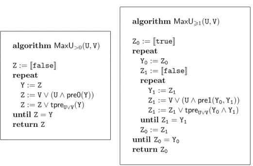
Figure 4: MaxU_>0 and MaxU_>1 algorithms

We first recall the results for computing maximum qualitative probabilities of finite state probabilistic systems, which requires the introduction of the following functions. For a prob- abilistic systemPS= (S,Steps,L⁰) and X, Y ⊆S let:

pre₀(X) = {s∈S| ∃(s, p)∈Steps.∃s⁰∈X.p(s⁰)>0}

pre₁(Y, X) = {s∈S| ∃(s, p)∈Steps.(∀s⁰∈S.(p(s⁰)>0→s⁰∈Y)∧ ∃s⁰∈X. p(s⁰)>0)}. Intuitively,s∈pre₀(X) if one can go fromstoXwith positive probability ands∈pre₁(Y, X) if one can go from s to X with positive probability and with probability 1 reach Y. Using these functions we have the following proposition¹.

Proposition 13 [dA97] If PS = (S,Steps,L) is a finite state probabilistic system and φ, ψ are PCTL formulae, then

• {s∈S|p^max_s (φ U φ)>0} equals the fixpoint µX.(ψ∨(φ∧pre₀(X)));

• {s∈S|p^max_s (φ U ψ)>1} equals the double fixpoint νY.µX.(ψ∨(φ∧pre₁(Y, X))).

We adapt this approach to probabilistic timed automata. First, using the functiondpre, the analogues of pre₀ and pre₁ for the discrete transitions of a PTA are given in Figure 3. It therefore remains to consider the time transitions of a PTA. For such transitions, we must take into account the state and formula clock valuation pairs that are passed through as time elapses. More precisely, for PTCTL, when using the time predecessor function we must ensure that we remain in the set of symbolic states satisfying φ∨ψ, that is, take the time predecessor tpre[[φ]]∨[[ψ]](·). Following this observation, Figure 4 presents the algorithms for computing{s,E |p^max_s,E (φU ψ)>0}and {s,E |p^max_s,E (φ U ψ)>1}.

In the case of computing quantitative maximum probabilities we use the approach de- scribed in [KNS01]. The algorithm is given in Figure 5. The key observation is that to

1See [BdA95] for the definitions of PCTL,p^max_s (φUψ) andp^min_s (φUψ).

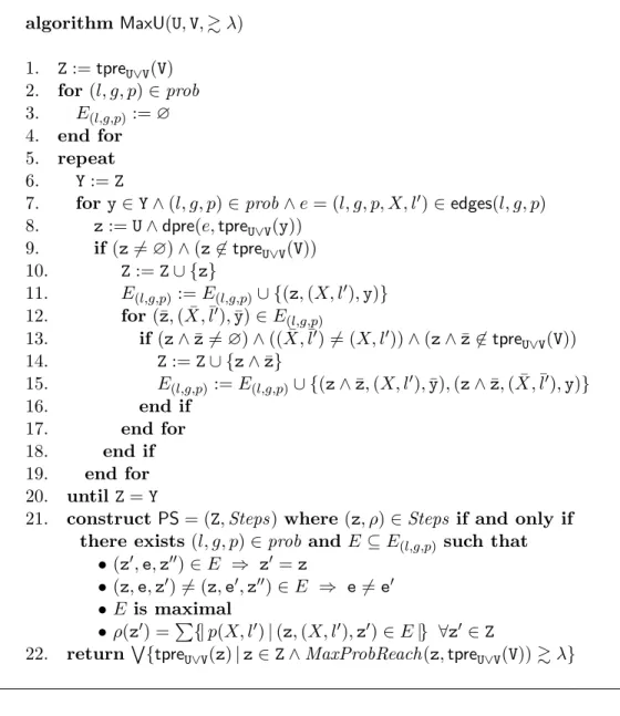
preserve the probabilistic branching one must take the conjunctions of symbolic states gener- ated by edges from the same distribution. Lines 1–4 deal with the initialisation ofZ, which is set equal to the set of time predecessors ofV, and the set of edgesE_(l,g,p)associated with each probabilistic edge (l, g, p)∈prob. Lines 5–20 generate a finite-state graph, the nodes of which are symbolic states, obtained by iterating timed and discrete predecessor operations (line 8), and taking conjunctions (lines 12–17). The edges of the graph are partitioned into the sets E_(l,g,p) for (l, g, p) ∈ prob, with the intuition that (z,(X, l⁰),z⁰) ∈ E_(l,g,p) corresponds to a transition from any state inzto some state inz⁰ when the outcome (X, l⁰) of the probabilistic edge (l, g, p) is chosen. The graph edges are added in lines 11 and 15. The termination of lines 5–20 is guaranteed (see [KNS01]). Line 21 describes the manner in which the probabilistic edges of the probabilistic timed automaton are used in combination with the computed edge sets to construct the probabilistic transition relationSteps. Finally, in line 22, model check- ing is performed on the resulting finite-state probabilistic systemPSto obtain the maximum probability of reachingtpre_U∨V(V) for each z∈Z. Note that we write z6=∅ if and only ifz encodes at least one state and formula clock valuation pair. The following proposition states the correctness of this algorithm.

Proposition 14 For any probabilistic timed automaton PTA, corresponding timed probabilis- tic system TPS = (S,Steps,L⁰) and PTCTL formula P_.λ[φ U ψ], if PS = (Z,Steps) is the probabilistic system generated byMaxU([[φ]],[[ψ]],&λ) then for any s,E ∈S×R^|Z|:

• p^max_s,E (φ U ψ)>0 if and only if s,E ∈tpre_[[φ∨ψ]](Z);

• if p^max_s,E (φ U ψ)>0, then p^max_s,E (φ U ψ) equals max

n

MaxProbReach(z,tpre_[[φ∨ψ]][[ψ]])

z∈Zand s,E ∈tpre_[[φ∨ψ]](z) o

.

Proof. See Appendix A. ut

Combining the above results we setUntil([[φ]],[[ψ]],.λ) equal to:

• [[true]]\MaxU_>0([[φ]],[[ψ]]) if.=6and λ= 0;

• [[true]]\MaxU_>1([[φ]],[[ψ]]) if.=<and λ= 1;

• [[true]]\MaxU([[φ]],[[ψ]],6&λ) otherwise.

As in the case of finite state probabilistic model checking, we can use the qualitative algorithms as precomputation algorithms when computing quantitative probabilities. In particular, we can setUntil([[φ]],[[ψ]],.λ), forλ∈(0,1), equal to:

[[true]]\MaxU(MaxU_>0([[φ]],[[ψ]])\MaxU_>1([[φ]],[[ψ]]),MaxU_>1([[φ]],[[ψ]]),6&λ). 4.3 Computing Minimum Probabilities

We now consider the problem of verifying formulae of the formP_&λ[φU ψ] which, using (3), reduces to computing p^min_s,E(φU ψ) for all state and formula clock valuation pairs s,E. As in the cases for (non-probabilistic) timed automata and (finite-state) probabilistic systems with fairness constraints, when considering properties which have universal quantification over paths/adversaries the standard algorithm can no longer be applied. For example, for

algorithm MaxU(U,V,&λ) 1. Z:=tpre_U∨V(V)

2. for(l, g, p)∈prob 3. E_(l,g,p):=∅ 4. end for 5. repeat 6. Y:=Z

7. fory∈Y∧(l, g, p)∈prob∧e= (l, g, p, X, l⁰)∈edges(l, g, p) 8. z:=U∧dpre(e,tpre_U∨V(y))

9. if (z6=∅)∧(z6∈tpre_U∨V(V)) 10. Z:=Z∪ {z}

11. E_(l,g,p):=E_(l,g,p)∪ {(z,(X, l⁰),y)}

12. for(¯z,( ¯X,¯l⁰),¯y)∈E_(l,g,p)

13. if (z∧¯z6=∅)∧(( ¯X,¯l⁰)6= (X, l⁰))∧(z∧¯z6∈tpre_U∨V(V)) 14. Z:=Z∪ {z∧¯z}

15. E_(l,g,p) :=E_(l,g,p)∪ {(z∧¯z,(X, l⁰),¯y),(z∧z,¯ ( ¯X,¯l⁰),y)}

16. end if

17. end for 18. end if 19. end for 20. untilZ=Y

21. constructPS= (Z,Steps) where(z, ρ)∈Steps if and only if there exists(l, g, p)∈prob andE ⊆E_(l,g,p) such that

• (z⁰,e,z⁰⁰)∈E ⇒ z⁰=z

• (z,e,z⁰)6= (z,e⁰,z⁰⁰)∈E ⇒ e6=e⁰

• E is maximal

• ρ(z⁰) =P

{|p(X, l⁰)|(z,(X, l⁰),z⁰)∈E|} ∀z⁰ ∈Z

22. return W{tpre_U∨V(z)|z∈Z∧MaxProbReach(z,tpre_U∨V(V))&λ}

Figure 5: AlgorithmMaxUntil(·,·,&λ)

any formula clockz ∈ Z, under divergent adversaries the minimum probability of reaching z>1 is 1; however, if we remove the restriction to time divergent adversaries the minimum probability is 0.

The techniques we introduce here are based on those for non-probabilistic timed automata [HNSY94], which we now recall. In [HNSY94], it is shown that verifyingφ∀U ψ(‘all divergent paths satisfyφU ψ’) reduces to computing the fixpoint:

µX.(ψ∨ ¬z.((¬X) ∃U(¬(φ∨X)∨(z>c))) (4) for any c∈ Ngreater than 0. The important point is that the universal quantification over paths has been replaced by a existential quantification, allowing one to ignore the restriction to time divergence in the verification procedure.

For the analysis of probabilistic timed automata it is convenient to consider, instead of

until, the dual, release, formula φ ∃V ψ (‘there exists a divergent path satisfying φV ψ’).

Using (4), it follows that verifying the formula φ ∃V ψ can be performed by computing the fixpoint:

νX.(ψ∧z.(X ∃U((φ∧X)∨(z>c)))). (5) Now, from the semantics of PTCTL and the dualityφU ψ≡ ¬(¬φV ¬ψ), we have, for any statesofTPSPTA and formula clock valuation E:

p^min_s,E(φU ψ) = inf

A∈Adv_TPSp^A_s,E(¬(¬φV ¬ψ))

= inf

A∈AdvTPS

1−p^A_s,E(¬φV ¬ψ)

= 1− sup

A∈Adv_TPS

p^A_s,E(¬φV ¬ψ)

= 1−p^max_s,E (¬φ V ¬ψ).

Therefore, to verifyP_&λ[φU ψ], it suffices to calculatep^max_s,E (¬φ V ¬ψ) for all state and for- mula clock valuation pairs. In the case whenλ=1, by replacing the ∃operator with ¬P_<1[·]

in (5), we arrive at the following proposition.

Proposition 15 For any positive c ∈ N and PTCTL formulae φ, ψ, if z ∈ Z does not appear in eitherφ or ψ, then the set {s,E |p^max_s,E (φV ψ)>1} is given by the fixpoint νX.(ψ∧ z.¬P_<1[X U ((X∧φ)∨z>c)]).

Proof. Consider any positive c∈N, PTCTL formulae φ, ψ, and z∈ Z such that zdoes not appear in eitherφorψ. To ease notation we let:

p^max_>1 (φ V ψ) ={s,E |p^max_s,E (φV ψ)>1}, and prove the proposition by showing:

1. the set p^max_>1 (φV ψ) is a fixpoint ofG₁(·, c);

2. if G₁(Y, c) =Y, thenY ⊆p^max_>1 (φV ψ)

where G₁(X, c) = ψ∧z.¬P_<1[X U ((X∧φ)∨z>c)]. First, since, for any X ⊆ S×R^|Z|, X ⊇ [[z.¬P_<1[X U ((X∧φ)∨z>c)]]] it follows that: X ⊇ G1(X, c) for all X ⊆ S×R^|Z|. Therefore, to prove thatp^max_>1 (φV ψ) is a fixpoint it is sufficient to show that:

G₁ p^max_>1 (φV ψ), c

⊇p^max_>1 (φV ψ). Now, by definition ofφ V ψ (see Section 3.3) we have that:

• For anys,E ∈S×R^|Z|, ifs,E |=φ∧ψ, thenω,E |=φV ψfor all paths ω∈Path_ful(s), and hences,E |=φ∧ψimplies s,E ∈p^max_>1 (φV ψ). It follows thats,E |= (φ∧ψ)∨z>c implies s,E |= p^max_>1 (φV ψ)∧φ

∨z>cand therefore, using Lemma 10, for any s,E ∈ S×R^|Z|:

s,E |=z.¬P_<1

p^max_>1 (φV ψ) U ((φ∧ψ)∨z>c)

⇒s,E |=z.¬P_<1

p^max_>1 (φV ψ) U p^max_>1 (φ V ψ)∧φ

∨z>c . (6)

• For any s,E ∈S×R^|Z| and ω∈Path_ful(s), ifω,E |=φ V ψ, thens,E |=ψ, and hence:

s,E ∈p^max_>1 (φV ψ) ⇒ s,E |=ψ . (7)

• As the satisfaction of PTCTL is with respect to divergent adversaries, for any s,E ∈

p^max_>1 (φ V ψ), there exists an adversary A such that, from s,E with probability 1, one

remains in p^max_>1 (φ V ψ) until either a state satisfying φ∧ψ is reached or more than c time units pass. Therefore, since the clock z does not appear in φ or ψ, for any s,E ∈S×R^|Z|:

s,E ∈p^max_>1 (φV ψ) ⇒ s,E[z:= 0]|=¬P_<1

p^max_>1 (φV ψ) U ((φ∧ψ)∨z>c) . (8) By definition ofG1:

G1(p^max_>1 (φV ψ), c) =ψ∧z.¬P_<1

p^max_>1 (φV ψ)U φ∧p^max_>1 (φ V ψ)

∨z>c

⊇ ψ∧z.¬P_<1

p^max_>1 (φV ψ) U ((φ∧ψ)∨z>c)

by (6)

⊇ ψ∧p^max_>1 (φV ψ) by (8) and Definition 9

= p^max_>1 (φ V ψ) by (7)

and hence p^max_>1 (φV ψ) is a fixpoint ofG1(X, c).

To complete the proof it remains to show that, if G1(Y, c) =Y, then Y ⊆p^max_>1 (φ V ψ) which we prove by contradiction. Therefore, suppose that there exists a of statesY such that G1(Y, c) =Y and p^max_>1 (φV ψ) ⊂Y. Now for any s,E ∈Y \p^max_>1 (φV ψ), and adversaryA, under A starting from s,E the probability of satisfying φV ψ is less than 1, and therefore the probability of satisfying the dual formula¬φU ¬ψ is greater than 0. It then follows that there exists a path ω ∈ Path^A_ful(s) such that ω,E |= ¬φU ¬ψ, and since z does not appear in eitherφ orψ,ω,E[z:= 0]|=¬φU ¬ψ. Hence, there exists some durationtA such that at some point along this path ¬ψ∧(z=t_A) is true and at all preceding points¬φ∨ ¬ψis true.

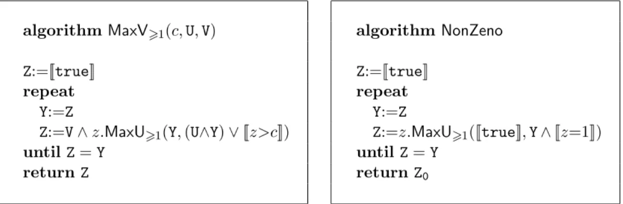
However, since s,E ∈ Y, and therefore s,E ∈ G₁(Y, c) it follows that there exists an adversary such that with probability 1 froms,E[z:= 0] one remains inY while z6c unless a state in Y which satisfiesφis reached. Since the above holds for any s⁰,E⁰ ∈Y and z does not appear inφorψ, iterating the above result, we have that for anyn∈Nwe can construct an adversary A⁰ such that, for anyn∈N, underA⁰ froms,E one remains inY whilez6n·c unless a state in Y which satisfies φ is reached. Furthermore, sinceY = G₁(Y, c) it follows that Y ⊆ψ, and hence under A⁰, for any n∈ N, with probability 1, from s,E one remains in states satisfying ψ while z 6n·c unless a state satisfying φ∧ψ is reached. From above, there exists some duration t_A⁰ and path ω⁰ ∈ Path^A_ful⁰(s) such that at some point along this path¬ψ∧(z=t_A) is true and at all preceding points¬φ∨ ¬ψis true. However, considering any n such thatn·c > tA (which exists since c >0) leads to a contradiction. ut The algorithm for calculating the set {s,E |p^max_s,E (φV ψ)>1} follows from Proposition 15 and is given in Figure 6. Note that we cannot use the same approach for calculating the set {s,E |p^max_s,E (φV ψ)>0}, i.e. in (5) replace∃with¬P₆₀[·]. This is because the greatest fixpoint in this case yields the set of state and formula clock valuation pairs for which, under some divergent adversary, there exists a path which satisfiesφ V ψ, which does not imply that the probability of satisfying φV ψis greater than zero.

Instead, we employ the following proposition, which together with Proposition 15 provides us with a method for verifying P_&λ[φU ψ] when λ∈[0,1).

algorithmMaxV_>1(c,U,V) Z:=[[true]]

repeat Y:=Z

Z:=V∧z.MaxU_>1(Y,(U∧Y)∨[[z>c]]) untilZ=Y

returnZ

algorithmNonZeno

Z:=[[true]]

repeat Y:=Z

Z:=z.MaxU_>1([[true]],Y∧[[z=1]]) untilZ=Y

returnZ0

Figure 6: MaxV_>1(c,U,V) and NonZenoalgorithms

Proposition 16 For any probabilistic timed automataPTA, corresponding timed probabilistic systemTPS = (S,Steps,L⁰), s ∈S, formula clock valuation E ∈R^|Z| and PTCTL formulae φ, ψ:

p^max_s,E (φ V ψ) =p^max_s,E (ψ U ¬P_<1[φ V ψ]).

Proof. Consider any PTCTL formulaeφ and ψand let A_max be an adversary such that for anys,E ∈S×R^|Z|:

p^A_s,E^max(ψ U (ψ∧φ)∨ ¬P_<1[2(¬φ∧ψ)]) =p^max_s,E (ψ U (ψ∧ψ)∨ ¬P_<1[2(¬φ∧ψ)])

and if one reaches anys⁰,E⁰ satisfying¬P_<1[2(¬φ∧ψ)], thenAmaxbehaves like the adversary Afor which:

p^A_s0,E⁰(2(¬φ∧ψ)) = p^max_s,E (2(¬φ∧ψ)) = 1

sinces⁰,E⁰ |=¬P_<1[2(¬φ∧ψ)]. Note that, this adversary is well defined (and divergent) since for any adversaryA, once a state satisfying¬P_<1[2(¬φ∧ψ)] is reached, the behaviour ofAhas no influence on the probability of satisfaction of the formulaψ U (ψ∧ψ)∨ ¬P_<1[2(¬φ∧ψ)].

Furthermore, for any s⁰,E⁰ such that p^max_s,E (2(¬φ∧ψ)) = 1, the fact that there exists an adversaryAsuch that p^A_s,E(2(¬φ∧ψ)) = 1 follows from Proposition 15.

Now, since for any s,E ∈S×R^|Z| and A ∈ Adv_TPS we have p^A_s,E(2(¬φ∧ψ)) = 1 if and only ifω,E |=2(¬φ∧ψ) for all ω∈Path^A_ful(t), it follows from the construction ofA_maxthat, for anys,E ∈S×R^|Z| and path ω ∈Path^A_ful^max(s), if ω,E |=ψ U (φ∧ψ)∨ ¬P_<1[2(¬φ∧ψ)], thenω,E |=φV ψ. Therefore, for alls,E ∈S×R^|Z|:

p^A_s,E^max(ψ U (φ∧ψ)∨ ¬P_<1[2(¬φ∧ψ)])6p^A_s,E^max(φ V ψ), and hence, by the definition ofA_max, it follows that

p^max_s,E (ψ U (φ∧ψ)∨ ¬P_<1[2(¬φ∧ψ)])6p^max_s,E (φV ψ) ∀s,E ∈S×R^|Z|. (9) On the other hand, from Lemma 12 and the fact that for anys,E ∈S×R^|Z| and adversary A: p^A_s,E(2(¬φ∧ψ)) = 1 implies s,E |= ¬P_<1[2(¬φ∧ψ)] we have for any adversary A and s,E ∈S×R^|Z|: p^A_s,E(ψU (ψ∧ψ)∨ ¬P_<1[2(¬φ∧ψ)])>p^A_s,E(φV ψ), and hence it follows that:

p^max_s,E (ψ U (φ∧ψ)∨ ¬P_<1[2(¬φ∧ψ)])>p^max_s,E (φV ψ) ∀s,E ∈S×R^|Z|. (10)

Combining (9) and (10) we have:

p^max_s,E (ψ U (φ∧ψ)∨ ¬P_<1[2(¬φ∧ψ)]) =p^max_s,E (φV ψ) ∀s,E ∈S×R^|Z|. (11) Now using (11) we have s,E |= ¬P_<1[ψU (φ∧ψ)∨ ¬P_<1[2(¬φ∧ψ)]] if and only if s,E |=

¬P_<1[φ V ψ], and since for any formulaeθ₁, θ₂ ands,E ∈S×R^|Z|: p^max_s,E (θ1 U θ2) =p^max_s,E (θ1 U ¬P_<1[θ1 U θ2]), using (11) again, we have:

p^max_s,E (ψ U ¬P_<1[φV ψ]) =p^max_s,E (φV ψ).

as required. ut

Combining the above results, we set Until([[φ]],[[ψ]],&λ) to:

• [[true]]\MaxV_>1(c,[[¬φ]],[[¬ψ]]) if&=> andλ=0;

• [[true]]\MaxU_>0([[¬ψ]],MaxV_>1(c,[[¬φ]],[[¬ψ]])) if &=>and λ=1;

• [[true]]\MaxU([[¬ψ]],MaxV_>1(c,[[¬φ]],[[¬ψ]]),>1−λ) if &=>and λ∈(0,1);

• [[true]]\MaxU([[¬ψ]],MaxV_>1(c,[[¬φ]],[[¬ψ]]), >1−λ) if &=>and λ∈(0,1).

4.4 Checking Non-Zenoness

We now consider how to check that the probabilistic timed automaton under study is non- zeno. In the non-probabilistic case checking non-zenoness corresponds to finding the greatest fixpoint νX.(z.(true ∃U ((z=1)∧X))). For probabilistic timed automata, we can replace

∃ with ¬P_<1[·], i.e replace ‘there exists a path that reaches (z=1)∧X’ with ‘there exists an adversary which reaches (z=1)∧X with probability 1’. Following this approach, the algorithm for calculating the set of non-zeno states is given in Figure 6. A probabilistic timed automata is then non-zeno if and only if the algorithm NonZeno returns the set of symbolic states [[true]]. Formally, we have the following proposition.

Proposition 17 A probabilistic timed automatonPTAis non-zeno if and only if{(l,inv(l)|l∈ L} equals the fixpointνX.(z.¬P_<1[true U ((z=1)∧X)]).

Proof. Consider any probabilistic timed automataPTAand suppose thatPS_PTA= (S,Steps,L) is the corresponding timed probabilistic system. To ease notation we let:

Snz= s∈S

Prob^A_s{ω∈Path^A_ful(s)|ω is divergent}= 1 for some adversaryA . We prove the proposition by showing that:

1. the set S_nz is a fixpoint ofG_nz(·);

2. if Gnz(Y) =Y, thenY ⊆Snz

(di,16x62∧z>6) (di,16x62∧z>3) (di,16x62) (si,26x63) (si,26x63∧z>3)

(si,26x63∧z>6)

(si, x63∧z>x+ 3)

(sr, z>6) (di, x62∧z>x+ 4)

0.1

0.9 0.1

0.95 0.05

0.05

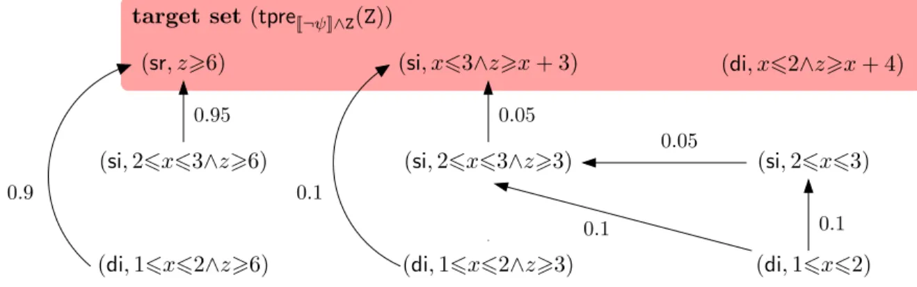
0.1 target set(tpre_[[¬ψ]]∧Z(Z))

Figure 7: Probabilistic system PSgenerated by the algorithmMaxU

where G_nz(X) = z.¬P_>1[true U (z=1)∧X]. First,S_nz ⊆G_nz(S_nz), and therefore to prove S_nzis a fixpoint ofG_nzit remains to show thatS_nz⊇G_nz(S_nz). Considering anys∈G_nz(S_nz), by definition ofGnz there exists an adversaryAunder which, with probability 1, from sone reaches a state inS_nz after 1 time unit. Therefore considering the adversary which behaves asA except that when a state in S_nz is reached, and in such a case the adversary lets time diverge with probability 1 (such choices exists by the definition ofSnz). It follows that, under this adversary, time diverges fromswith probability 1, and hences∈Snz as required.

It therefore remains to show that, if G_nz(Y) = Y, then Y ⊆ S_nz which we prove by contradiction. Therefore, suppose that there existsY such thatGnz(Y) = Y and Y ⊃ Snz. Now, by definition of Snz, if s ∈ Y \Snz there does not exist an adversary for which time diverges fromswith probability 1. However, sinceG_nz(Y) =Y, there exists an adversary for which with probability 1 one reaches a state in Y after 1 time unit. Iterating this fact, we have that for any n∈N, there exists an adversary which with probability 1 reaches a state inY after ntime units. Therefore s∈S_nz which is a contradiction. ut Similarly to [HNSY94], the algorithm can be used to convert a ‘zeno’ probabilistic timed automaton into a non-zeno automaton by strengthening invariants. More precisely, supposing NonZeno returns Z, we can construct a new invariant condition by letting inv_nz(l) = ζ_Z^l for each locationlof the automaton under study.

4.5 Example

We now return to thePTAin Figure 1 and verify the propertyz.P_>λ[φU ψ], whereφ=true andψ= (sr∧z<6), which involves computing the set of states for which minimal probability of a message being correctly delivered before 6 time units have elapsed is greater than λ.

In particular, we consider this minimum probability when starting from the locationdi with the clock x equal to 0. In particular, we consider the minimum probability of correctly delivering before 6 time units have elapsed starting from the location di with the clock x equal to 0. In this example, we do not distinguish between the name of a location and the atomic proposition with which it is labelled. According to our methodology, the set of states satisfyingP_>λ[φ U ψ] is given by the following set of symbolic states:

[[true]]\MaxU([[¬ψ]],MaxV_>1(c,[[¬φ]],[[¬ψ]]),>1−λ).