Application to Aircraft Design

A análise aerodinâmica é realizada pelo método do painel 3D e a análise estrutural pelo método dos elementos nitos, ambas implementadas por ferramentas de análise externas, cuja interação é realizada pela aplicação desenvolvida. Palavras-chave: Projeto Ótimo Multidisciplinar, Otimização por Enxame de Partículas, Redes Neurais, Método de Painel Tridimensional, Método de Elementos Finitos, Frente de Pareto.

Introduction

Thesis Objective

Thesis Layout

In Chapter 3, a historical perspective on Evolutionary Algorithms is given followed by the selection and development of the optimizer algorithm to be used (Particle Swarm Optimization) in the MDO application. Finally, in chapter 9, conclusions are drawn from the results presented in the previous chapters and the completion of the proposed objectives is discussed.

Introduction

Ideally, the MDO environment should be interactive and flexible enough to allow the problem constraint, constraint enforcement, and simulation depth to be fully specified by the design team, rather than individual discipline teams. Although process allocation can present some management challenges, it really allows allocation to be a physical resource allocation, rather than just a process allocation.

MDO Strategies Applied to Aircraft Design

In this work, it is shown that one of the major challenges in performing MDO is being able to. The main objective of the work itself was to analyze the robustness of the particle swarm algorithm.

Introduction

Particle Swarm Optimisation

• Implementation of the PSO
• Detailed Implementation
• Validation of the Implemented Optimiser

Again, the choice of its value should be made taking into account the desired behavior of the herd. The herd then simply consists of a vector of n individuals of the type defined in the class.

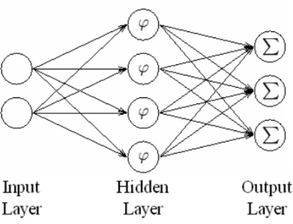
Articial Neural Network

• Accelerator for the PSO
• Pareto Front Detection

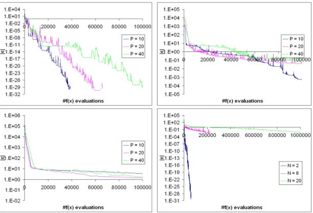
From the results shown, we can conclude that the optimizer is able to find the minima (although not always the global minimum) of the considered test functions. In terms of timing and overall application, we can expect the optimizer's operations to have almost no impact. The solution should be able to shorten the most time-consuming process, ie. determining the value of the objective function.

Section 4.2 explains a description of the chosen method, the 3D Panel Method, and its computational implementation.

Introduction

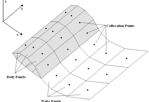
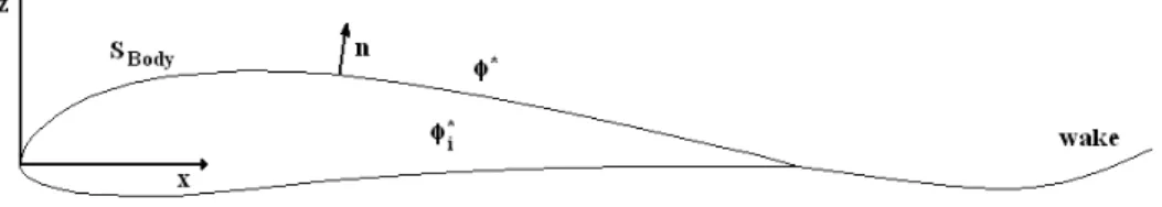
For its balance between precision and computational cost, the 3D panel method was chosen as the aerodynamic solver for this work. These considerations mainly concern the proper modeling of the wake (the three-dimensional equivalent of the Kutta condition [38]). Their positioning depends on several factors, such as the chosen model for the singularities themselves and the degree of the method.

CMARC is an improved version of the Panel Method Ames Research Center (PMARC) code, developed by NASA Ames Research Center, as a low-order panel method that supports complex geometries.

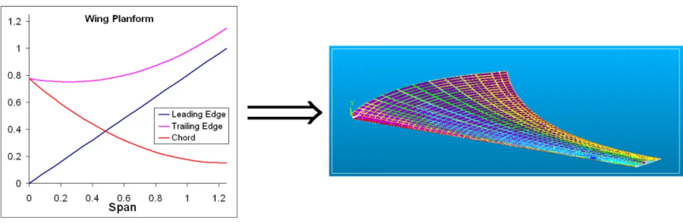
Aircraft Parameterisation

• Wings and Stabilizing Surfaces
• Fuselage and non-Lifting Bodies

Constraints can and should of course be applied to any of the design variables so that any physically imposed constraints are carried over to the aerodynamic model. By having the values ​​of the design variables, the parameterization of the panel's corners can be done. Parameterθj is the angle of a section j in planyz, calculated from the derivative of the dihedral as a function of the span.

Additionally, it is critical that there are no overlapping or crossing panels as there must be a clear definition of what is the inside and outside of the model.

Analysis Options and Solution Post-Processing

It is possible to include any body as a lifting body in the 3D Panel Method, provided that a suitable wake is created. This fact and considering that, from an aerodynamic design point of view, the airframe should generally generate as little lift as possible (ideally, none at all, since the induced drag component is very high compared to that of a wing) , it was decided not to include a wake in the body, making it a non-lifting body. Aircraft concepts such as Boeing's Blended Wing Fuselage or United Wing Aircraft, in which the fuselage obviously plays an important role in relation to lift generation, should not be treated in this way, which is suitable for more traditional aircraft design.

Then, in Section 5.2, a thorough description of the FE model is made, followed by some aspects of load application to this model, in 5.3.

Introduction

Structural Model

• Wing and Fuselage Panels
• Spars
• Ribs, Stringers and Stieners

In this case, it makes sense to use the discretization of the aerodynamic module as a starting point for the FE model. This allows the information from the aerodynamic analysis output file to be used to create the outer panels of the aircraft. The principle of construction under tension is based on the fact that the cladding, i.e. outer panels of the structure, withstands most of the stresses arising from aerodynamic loads.

The spanwise distribution of thickness along the shear web and the chordwise position of the spar(s) are the design variables.

Structural Loads

Solution Post-Processing

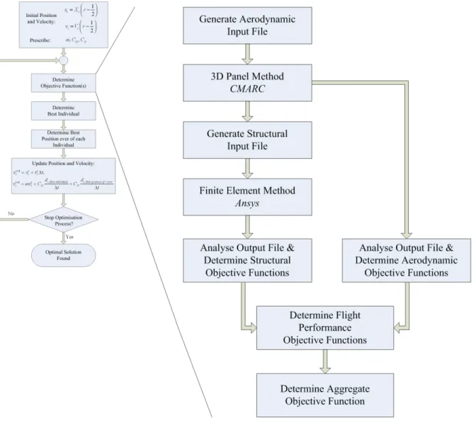
The following sections will present the steps taken in the development of the application, in the same order as they were taken, and at the end of this chapter, a flow chart of the application is presented.

Introduction

Implementation of the Optimisation Algorithm

• Denition of the Optimisation Vector
• Swarm Denition
• Scattering of the Initial Swarm

Moreover, even a radical redesign of the class and the functions it contains has absolutely no effect on the developed code for the optimizer operations. Defining the boundaries for each component (6.1) and defining the number of individuals in the swarm will determine the initial convergence behavior of the algorithm. Becoming sensitive to this issue was something that happened on the job and can be considered part of the learning curve for anyone working in this field.

Therefore, and only as a rule of thumb, the velocity initial space is dened as an amplitude between 10% and 20% of the amplitude for the position initial search space, in each direction.

Individual Class Functions

• Objective Function
• Best Ever Objective Function

Then, all station point coordinates are declared for all patches, specifying whether the patch has a symmetric correspondent. Finally, all les that are not needed in subsequent blocks of the application are deleted, a feature that will also be used after the structural production analysis of the les. This block is similar to the one for the aerodynamic analysis, being simpler, as it only includes the AnsysR run call followed by the name of the previously generated let input.

After all the functions contributing to the AOF have been determined in the blocks above, and according to equation (3.8), the AOF is simply calculated by doing a weighted sum of all the contributing objective functions.

Enhancements to the Optimisation Process

• Limiters
• Global to Local Search: Inertia and ∆t

Another implemented feature was to change the characteristics of the swarm, regarding its search behavior. Therefore, the chosen strategy was to start with an inertia value close to unity and slightly decrease the inertia of the particles with time. As the inertia gradually decreases, the swarm converges faster to the minimum within the region where the global minimum is, i.e. it converges rapidly to the global minimum.

These, two in the aerodynamic field and two in the structural field, were used to test the developed application in the context of real-life problems, but also to increase knowledge about the behavior of the optimization process as a whole.

Aerodynamic Optimisation

• Rectangular Wing Optimisation
• Winglets Optimisation

The strategy is to create a set of ailerons that will increase the aircraft's performance while maintaining the aircraft's original stability as much as possible. The objective of the optimization problem is to increase the basic L/D ratio without changing the CM of the aircraft. This provides the initial static stability by applying a penalty if the pitching moment of the aircraft changes;

Figure 7.5 shows the evolution of the optimization process, where the objective function value is shown for each of the six individuals in the swarm during the prescribed eight time steps.

Structural Optimisation

• Beam Optimisation
• Shell Thickness and Ribs Optimisation

It shows the effect of having a component in the objective function that benefits solutions where this element is loaded in a uniform manner. Finally, Figures 7.13 and 7.14 show the evolution of the objective function and mass for this optimization problem. In this problem, the overall objective function considered mass, tip rotation, tip detection, and maximum verified stress.

Nevertheless, the algorithm was able to minimize the objective function to what appears to be the optimal point, since the best individual's mass shows a convergence behavior.

Lessons Learnt with Singleobjective Optimisation

It should also be noted that the mean values ​​of the herd also show a convergence towards the best individual, a behavior that also suggests that the optimum point has been reached.

Statement of the Problem

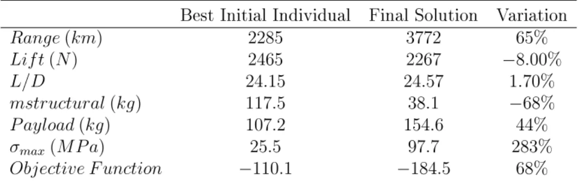
Recalling (4.8) and considering sep= 2, this represents a total of 13 ac parameters that are optimized. The parameter Wi is calculated from the lift obtained from the aerodynamic solution and evaluated. In this problem, the aggregate objective function was constructed to evaluate each solution considering primarily the range, but also included other functions to ensure that the wingtip displacement and rotation, the maximum stress in the structure, and the peak moment were within bounds. , in one approach. similar to what is stated in sections 7.1.2 and 7.2.2.

Results

Analyzing only aerodynamic performance in lift and L/D ratio shows two similar solutions, but their differences emerge when the results of the structure are considered. However, the optimal incidence distribution combined with the accentuated backswing of the wing has a balancing effect on the aircraft with respect to the pitching moment, guaranteeing static stability. As expected, the wing root region exhibits higher stresses than the rest of the structure, especially near the leading edge, as not only upward bending occurs due to lift, but also rearward bending due to drag.

A modular approach has also proven useful, as changing the complexity of the model or analysis tools has no impact on the rest of the application.

Conclusions

The nite element model is derived from the output of the aerodynamic solver, guaranteeing the best possible fit between the aerodynamic and structural models. It should be noted that the main goal of the work described in this document was to develop a framework based on the MDO methodology. As for future developments, perhaps one of the most interesting concepts that can be applied to this type of application is distributed computing.

To perform this detailed analysis, a preliminary solution must obviously be produced, and that is the primary task of the present application.