Hydrodynamic analysis of a slalom fin of windsurf board

The aim of this thesis is to perform a hydrodynamic analysis in estimating the water-induced loads on a real slalom fin of a windsurfing board. First, an initial 2D flow study of the fin support hydrofoil will be carried out using the software XFOIL.

List of Tables

Nomenclature

Glossary

Introduction

• Motivation
• Objectives
• Thesis Structure
• Conceptualisation and State-of-the-Art

Despite the comprehensive checklist, the study will focus on the analysis of the flow around the SFWB. Depending on the user, conditions and type of windsurfing, the sail area may vary.

Slalom Fin of Windsurf Board

• Work Description
• Bibliographic Revision
• Work Case Studies
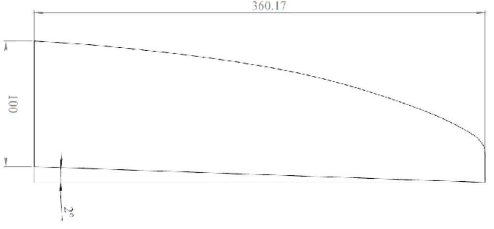
• Fin Design and Physical Properties
• Aerofoils
• Navier-Stokes and CFD Analysis
• Boundary Layer

To complete the research, the 3-D analysis of the complete fin will be run on Star-CCM. The Reynolds number is based on the minimum and maximum length of the SFWB chord, and is very sensitive to this value. In this particular case, it is the cross-section of the windsurf board's fin, also named as a hydrofoil.

The leading edge is the point at the front of the airfoil that has the greatest curvature. The trailing edge is the point of greatest curvature at the rear of the wing. Thus, there is suction on the upper surface and pressure on the lower surface, all of which contribute to the creation of aerodynamic force.

What is expected from the Navier-Stokes equations is the interaction of the flow with the airfoil surface.

Preliminary Analysis

• Initial Considerations
• Pre-Analysis Software Selection
• Case Study 1
• Initial Stage
• Analysis
• Case Study 2
• Results Discussion

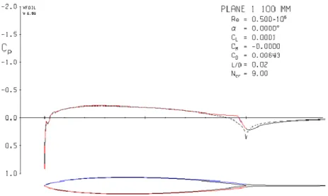
At this point, only half of the profile is drawn, as the hydrofoil is symmetrical. Based on the observed consistency of the results from the last chapter, it is assumed that the program is being used correctly. The pressure coefficient distribution (example in Figure 3.8), plotted to represent the dimensionless surface pressure, shows, as expected, a maximum value at the top of the profile at zero degrees.

However, with respect to this distribution, a smoother slope was noticeable very close to the tip of the hydrofoil at the top. It is seen to increase as the angle of attack increases, parallel to the growth of the exposed area, in the path of the streamlines. On the upper surface, the flow remains laminar up to 97 % of the chord at 0°, then around 2°, the separation point shifts abruptly to the leading edge, about 4 % of the chord.

In conclusion, a transition on the top surface of the foil is expected, as it repeats for low Re.

Mesh, Turbulence and Transition Model

• CFD Software Selection
• Star-CCM+ Aerodynamic Models
• SST k – ω Turbulence Model
• Mesh Characteristics
• Case Study 3
• Validation Conclusions

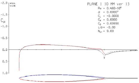
The cord length defined is 100 mm, which is equivalent to the length at the root of the SFWB. The k – ω SST model shows a slightly higher value for the peak of the curve, with a maximum error of 6. The results of the k – ω SST model without the transition addition can be explained due to the nature of the model itself.

However, it changes about half of the hydrofoil, where the flow will have a turbulent mode (intermittency of 1). Finally, Figure 4.4 verifies the above, where the turbulent kinetic energy has a peak around the end of the LSB, signaling reattachment of the flow to the turbulent boundary layer. Using the visual tools from Star-CCM+, an estimate of the transition location is presented in Figure 4.6.

This chapter ends with a preview of the necessary models and instructions for the following chapters.

SFWB Profile Performance

Case Study 4: SFWB Results

As expected, the variance is more significant near the leading edge, due to the fluctuation of the fluid and the point of separation. Also of relevant value is the variance near the trailing edge, which is expected as soon as turbulence will occur if the liquid leaves the pressure side of the foil. In parallel, to help visualize the shape of the turbulent field, the Q-criterion is shown in Figure 5.3.

For the leading edge, at b), the bubble seen on the pressure side is not an actual bubble, but only a characteristic of the flow impinging on the wall, stagnating and accelerating around it in the -i direction (Figure 5.7). a) Recirculation bubble at the trailing edge. The actual laminar separation bubble is on the suction side and measures at 4 degrees approx. 4% of the chord length. This may be due to the number of cells on Star compared to the length of the panels on XFOIL.

Because in the first seconds of the simulations, the foil causes a significant disturbance in the flow, a detailed pressure analysis is done.

Mesh Convergence Study

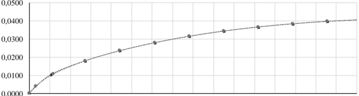
The simulations start from the implicit unstable state, 2nd order, and at a time step of 0.01 and 60 iterations. For the rest, the time step and the number of iterations per time steps are increased to 0.001 and 80, respectively, to obtain converged values. The last mesh, M7, goes beyond the possibility of having a difference in drag coefficient of 7% to the finer mesh.

It is noticeable that the drag coefficient is also the most delicate factor to study, perhaps because it is measured in the i direction, and here the number of cells decreases more significantly. In other words, the number of cells transverse to the foil is significantly less than the number of cells longitudinally, so increasing the cell size will reduce the number of cells, resulting in a worse result. So the grid parameters to use are those with a smaller number of cells but still within the 5% error margin.

It should be noted that having a less refined mesh will improve the computational time, but on the other hand, it takes a toll on the results.

General Conclusions

SFWB Operation

Physical models and mesh considerations

If not required, the time step and the number of inner iterations are not changed.

SWBD Three-Dimensional Aerodynamic Analysis

When drawing the coordinates for the 2-D hydrofoil, a gap formed on the trailing edge, which we then closed with a semicircle. A small band is expected immediately after the LSB and at the point where the pressure increases in Figure 6.3, near the trailing edge. As we move down Z, we see that the TKE isosurface fades out and reappears at the tip of the fin.

In Figure 6.6 it is essential to mention the higher values ​​of skin friction at the leading edge, and also a small and thin band near the trailing edge. It is also seen how higher friction values ​​are at the collar, in the same place where in Figure 6.5 the TKE blue band is found. For higher AoAs, the formation of a spiral vortex at the foil tip would be expected.

The blue color on the flow lines indicates that the flow is slowing down, which is represented at the leading edge (stagnant flow) and on the back half of the fin, near the tail.

General SFWB Conclusions

Additional Studies

Parametric Optimisation Study

• Maximum Thickness Position Variation
• Conclusions

For Cd (b), the +5% thickness case shows a very similar behavior, while the reduced thickness case shows more resistance (about 10% between 5 to 9 degrees). Regarding the separation point (c), almost no difference is felt on the underside (LS), but at small angles of attack the flow separates later. For the upper side (US), the separation point will move to the leading edge about 2 degrees, against 3° as in the previous analysis.

The significant difference to the previous plots is in Figure 7.4 (c), where the separation is taking place at the same AoA, on the upper surface. There is still gain for lower angles, where separation is occurring further up the chord. Unless it is proven preferable to have such properties, there is no point in implementing any of the modifications.

The results show a larger lift for small angles, but an earlier stall, with an increase in drag and earlier flow separation.

User Profiles

This also shows that the fin must be very carefully adjusted in terms of thickness, otherwise performance can be affected. Average user profile: This user has more experience than the basic user and can therefore achieve higher speeds. Master User Profile: the master user usually sails at high speeds and can also perform maneuvers.

The idea behind it is that for every angle of attack plus speed, pressure is found. Finally, the Weibull distribution or cumulative frequency of each pressure for each sailing case is plotted (Figure 7.5). a) Basic user (b) Average user (c) Power user. As expected, the basic user shows a higher probability of generating smaller pressure on the fin.

For the remaining users, the slope shifts to a more significant pressure, which is an indication of how each profile manages its speed/angle and associated pressure interval.

Notes on Water Tunnel Results

Conclusion

In this way, the mesh dimension around the sheet can be fine-tuned, to meet the needs of the physics model and to present quality results. The results with the SFWB hydrofoil revealed that there was, in fact, a recirculation bubble that the XFOIL failed to represent. After intensive searches, the only vortices were created where in the early stages of the simulation, before the solution converged.

The flow is believed to have instability, especially for larger AoAs, but one or both of the following possibilities may occur: either the mesh is too coarse to capture an instability phenomenon such as a Kelvin Helmholtz, or an unknown error occurred during simulation . Although the first goal was to use the mesh parameters closer to the previous simulations, it proved difficult to include the third control volume that added a very fine mesh to the leading and trailing edges of the fin. Finally, the parallel research in Newcastle at the cavitation tunnel shows that the fin stops at approx. 8° of AoA, a number satisfied by this thesis' simulations.

It also shows that the most critical force in the force resultant, measured in the SFWB, is the lift.

Future Work

Lienhard, “Thermophysical properties of seawater: A review and new correlations incorporating pressure dependence,” Desalination, vol. MCGhee, Experimental Results for the Eppler 387 Airfoil at Low Reynolds Numbers in the Lagley Low Turbulence Pressure Tunnel, NASA TM. Volker, "A correlation-based transition model using local variables - Part I: model formulation," Journal of turbomachinery, vol.

Appendix A

P113 Coordinates