Intelligent Traffic Light Management for Automated Guided Vehicle Systems using Deep Reinforcement Learning

We trained and tested three RL methods namely Deep Q-Network (DQN), Double DQN and Dueling DQN. We implemented and tested six scenarios with different numbers of lanes and phase configurations of traffic lights.

Context

Objectives

Document structure

Introduction

Main elements of an RL system

Kinds of RL algorithms

Markov Decision Process

To do this, Markov Reward Processes (MRP) expand the MP from to , with R and γ representing the reward discount function and factor, respectively. To represent that different impact, the concept of discounted return is introduced (Equation 2.5), where the reward discount factor (γ ∈[0,1]) is applied to reduce the impact of the previous steps.

Q-Learning

The agent uses these values ​​to choose the best action for each state. In the same equation, α∈[0,1] is the learning rate used by the agent in each iteration of the q-value update, is the reward obtained by taking action states, and γ is the reward discount factor.

Deep Q-Networks

Summary

Then, in section 2.4, we explained Markov decision processes (MDP) as they are useful for formalizing RL problems. Finally, in section 2.5 we briefly explained what q-learning methods are, and in section 2.6 one can understand how deep learning is used in combination with q-learning to achieve better results.

Introduction

The Alan Turing Institute’s TSC

ATI-TSC used a state vector with a dimension equal to the number of input lanes of the intersection plus one. The operation space used by ATI-TSC varies according to the complexity of the intersection. The main idea is that each action corresponds to the light phase of the traffic signal.

Two experiments were performed using the "cross triple" scenario, one with four phases and the other with eight. According to ATI-TSC, the same value of queue length in meters used for states is a reasonable choice for the reward function. The following equation (3.1) is the reward function used, where the reward of each step is the negative sum of lane queue lengths in meters.

IntelliLight

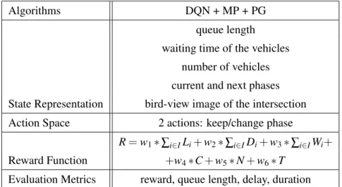
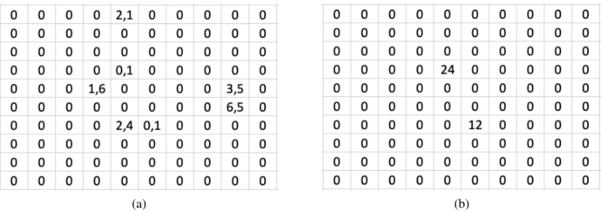
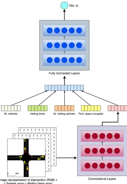
In addition to these, the condition includes a bird's eye view image of the junction (M), current light phase (Pc) and next light phase (Pn). A graphical representation of the state is seen as the input to the Q network in Figure 3.4. The delay is defined in equation 3.3, where the speed in the lane is the average speed of the vehicles, and the speed limit is the maximum speed allowed in that lane.

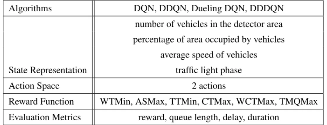
WWWiii is the sum of the waiting times of all vehicles j∈Ji in each lane (Equation 3.4). TTT is the total travel time (in minutes) of the vehicles that have passed through the intersection since the last agent actiona. Table 3.3 is an overview of the previous subsections, where one can see the algorithms, state representation, action space, reward function, and evaluation metrics that the IntelliLight authors used in their experiences.

CTLCM

CTLCM 19

Reward function WTMin, ASMax, TTMin, CTMax, WCTMax, TMQMax Evaluation metrics reward, queue length, delay, duration. Regarding the reward functions, it is possible to draw two conclusions: WCTMax provides less CO2 emissions and fewer waiting vehicles, and although TMQMax is the one with the most emissions, it is by far the one with the least waiting time.

Summary

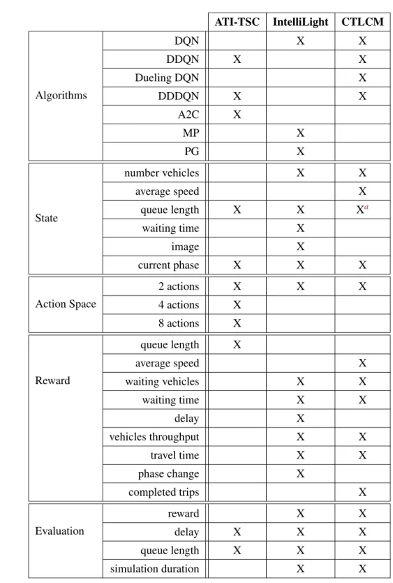
The first is that state representation must have the traffic lane lengths and the current phase of the traffic lights. The second is that the delay of vehicles and the sum of queue lengths in each step are good measures to evaluate the performance of the systems. Another important fact is that they all use as little action space as possible.

When analyzing the state representation of each solution, IntelliLight only used bird's-eye views of the intersections. Combined with other features such as queue length and the current traffic light phase, it optimizes the policy learned by the agent. Finally, when looking at the reward functions of the methods, there is no right way to go.

Problem Formalisation

Action space (A)— For action space, we use an integer value that indicates the next phase of the traffic light. Phases are different possible combinations for green/red traffic lights and are predetermined for each trial. Reward function (R) — The main objective of the reward function is to penalize collisions between vehicles while maintaining high traffic flow.

This is one of the most critical factors of the reward function because higher speeds directly lead to higher traffic flow. Ultimately, it is a wise choice to let this penalty grow linearly with the average speed of the vehicles. Changing the phase of the traffic light has a direct impact on near-future rewards, but not distant rewards.

Methodology

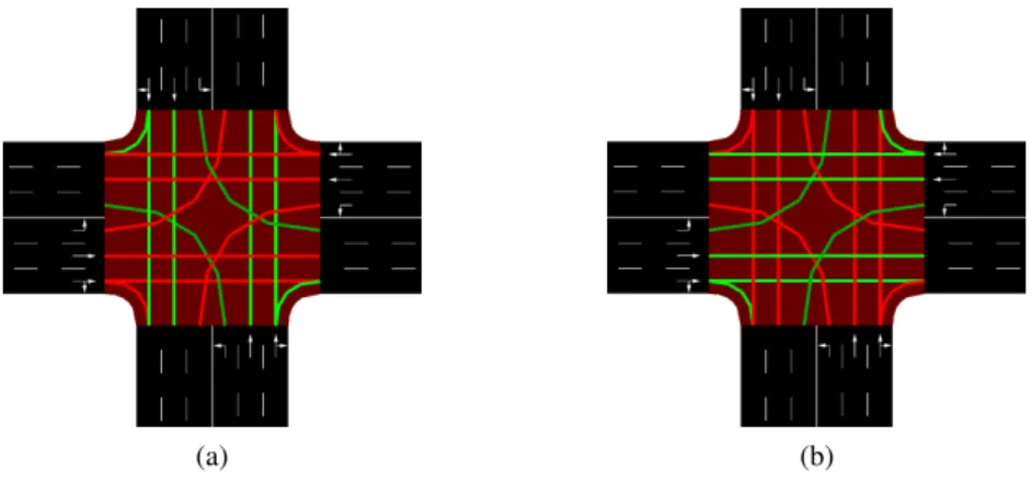
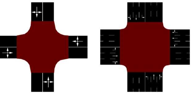
In this setup, there is actually a third phase that blocks traffic from all directions to let the agent clear the intersection if he wants to. Finally, the intersection with one-lane roads has a configuration with 4,096 phases, and the intersection with 3-lane roads has a configuration with 65,536 phases. Both of these setups allow the agent to control each line of motion individually (represented by the green and red lines in figures 4.6 and 4.7).

Every time the agent has to choose an action, a random number between 0 and 1 is generated. By exchanging information with SUMO, the environment builds the new state representation described in the previous section, calculates the value/reward of this state and sends this information (state and reward) back to the agent. This step is only processed after 64 steps of simulation to have enough tuples to perform batch training of the agent.

Simulation architecture

Having thoroughly researched several projects that use RL to control traffic (for example, the one in Chapter 2), SUMO [12] has become a widely used traffic simulator due to SUMO's Traffic Control Interface (TraCI). TraCI helps to exchange information about the environment with the agents and enables simultaneous use of a Graphical User Interface (GUI). The GUI is the part that allows us to collect images of the intersections at each step to build our state representation (Section 4.1).

It is possible to interact with the GUI through TraCI, creating a view at the center of the intersection and taking screenshots of this view at each step. Screenshots can be saved to the desired location and used by the program to build a national representation. Along with the images, TraCI allows us to collect a large amount of simulation data and change the state of the simulation as we wish (extensively.

Summary

This chapter is divided into two main sections: Section 5.1 discusses the results of the training pipeline loop (Subsection 4.2.2), and Section 5.2 discusses the results of the testing pipeline loop (Subsection 4.2.3).

Training

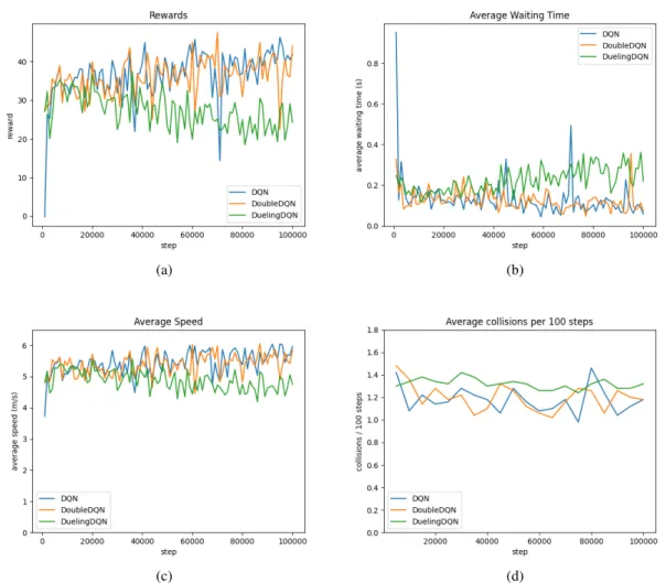
If we now analyze the scenario where we have single-lane roads and the traffic light has four phases (Figure 5.2), the Dueling DQN agent again gets the worst overall results. The scenario with one-lane roads and a traffic light with 4,096 phases is the most challenging for agents, as the action space is greatly increased. Comparing this scenario with the single-lane scenario in Figure 5.2 (page 36), all agents managed to be more stable and achieve better results.

Again, due to the size of the action space in this scenario, Figure 5-7 shows the agent's distribution of actions during training. As can be seen in the equivalent scenario with single lane roads (Figure 5.3 on page 37), Double DQN explores more actions than DQN because it chooses actions from the network that is not constantly updated. The Dueling DQN distribution shows that while it had some preference for some actions over others, it still did a decent amount of exploration of the action space.

Testing

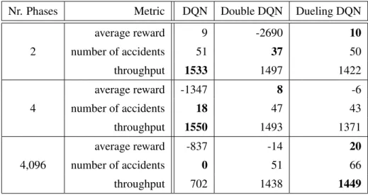
Comparing Double DQN with Dueling DQN, choosing which one is better is not easy. Double DQN still manages to be a good choice, especially in scenarios with large spans. All agents managed to keep the intersection crash-free with similar throughput in the two- or four-stage scenarios, which is excellent.

Dueling DQN rewards are lower than other agents due to the speed and waiting time of the vehicles. Both the DQN and Double DQN agents managed to keep the intersection free of long queues of vehicles (constantly under five vehicles), while the Dueling DQN agent occasionally formed a large queue on one of the roads, but only for short periods. Double DQN followed the same strategy of always keeping the same phase, but with a different combination of green and red lights.

Summary

Finally, Table 5.2 shows that increasing the traffic light's number of phases is not sufficient to keep traffic flowing.

Main Contributions

Future Work

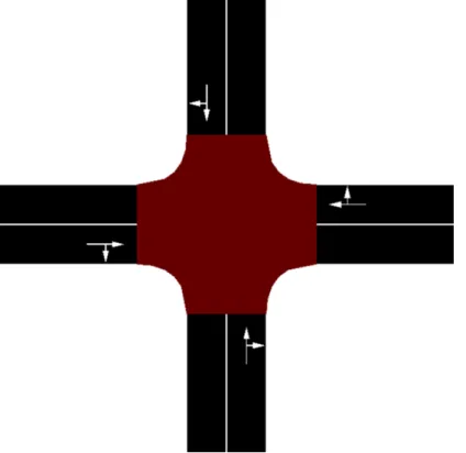
Although images bring many features with low programming effort, most of the pixels in these images are irrelevant. After a rough analysis of Figure 4.2(p.24), we can see that about 60% of the image represents the road environment, which is irrelevant for controlling the traffic light. The benefit of turning and rotating traffic situations is that from a single observation of the environment it is possible to generate eight different (but similar) states that our RL agents must be able to handle.

From real scenarios, we know that when we have multiple traffic lights in a more or less complex road network, the state of one traffic light can affect the traffic of the surrounding people. In these scenarios, the goal is not to optimize the traffic flow of each intersection individually, but to optimize the traffic flow of the entire road network. The five main challenges are partial observability of each agent, non-stationarity of the environment, handling of continuous action spaces, multi-agent training schemes so that all agents train together, and transfer of learning in multi-agent systems.