Appropriate management of such structures requires automated structural health monitoring (SHM) approaches to infer the actual state of the system. The superiority of the proposed approaches compared to the state-of-the-art is attested on standard datasets from monitoring systems installed on two bridges: the Z-24 bridge and the Tamar bridge.
Context
Without such data normalization procedures, varying operational and environmental conditions will produce false-positive indications of damage and rapidly erode confidence in the SHM system. Therefore, for statistical modeling phase, several machine learning algorithms with different working principles have been proposed (WORDEN; MANSON, 2007; FIGUEIREDO et al., 2011).
Related work
Traditional approaches for damage detection
KHOA et al., 2014) proposed an unsupervised adaptation for dimension reduction and damage detection in bridges. CHENG et al., 2015) applied KPCA to detect damage to concrete dams subject to normal variations.
Cluster-based approaches for damage detection
Similarly, novelty detection methods were proposed in (OH; SOHN; BAE, 2009; YUQING et al., 2015) by applying KPCA as a data normalization procedure. In (SANTOS et al., 2016a), a genetic-based approach is used to drive the EM search towards the global optimum.
Justification
A two-step damage detection strategy based on GMMs was developed in (FIGUEIREDO; CROSS, 2013; FIGUEIREDO et al., 2014b; SANTOS et al., 2016a) and applied to the long-term monitoring of bridges. To overcome the limitations imposed by EM, in (FIGUEIREDO et al., 2014b) the parameter estimation is performed using a Bayesian approach based on a Markov-chain Monte Carlo method.
Motivation
Objectives
Improve the literature of relevant SHM to damage assessment and identification by comparing the proposed methods with traditional methods. Apply the proposed methods to data sets of real structures subject to strict linear/non-linear effects, as a means of testing their performance and making comparisons.
Original contributions
The results indicate that the proposed approaches have overcome the traditional ones in terms of damage classification and robustness to deal with nonlinear effects caused by normal variations. Furthermore, the proposed cluster-based algorithm proves to be able to provide physical interpretations of structural conditions, enabling a better understanding of operational and environmental sources of variability.
Organization of dissertation
What are the conditions, both functional and environmental, under which the system to be monitored operates. It enables the reduction of time and cost efforts during the back-end stages, allowing the determination of the appropriate features to be extracted from the system being monitored and efforts to exploit the unique features of the damage to be detected.

Data acquisition
In this regard, the operational assessment seeks to establish limits and restrictions on the type of monitored parameters, aiming to determine how the monitoring will be carried out. Otherwise, the later stages would be performed without any reliability in the designed monitoring system.
Damage-sensitive feature extraction
The parameters of these models, or the associated predictive errors, become the damage-sensitive features.
Statistical modeling for feature classification
Linear principal component analysis
In the field of SHM, PCA is used for various purposes (feature selection, feature cleaning and visualization). The eigenvectors associated with the higher eigenvalues are the main components of the data matrix and correspond to the dimensions that have the greatest variability in the data. Precisely by choosing only the first eigenvectors, the final matrix can be rewritten without significant loss of information in the form of .
Auto-associative neural network
On the other hand, if the feature vector comes from the damaged state, the residual errors increase and the DI deviates from zero, thus indicating an abnormal state in the structure. In this work, the threshold is determined for 95% confidence in DIs considering only the basic data used in the training process. Thus, if the approach has learned the baseline condition, then about 5% of misclassifications in DI derived from undamaged observations not used for training are statistically guaranteed.
Kernel principal component analysis
The optimal value of 𝛾 can be estimated by requiring that the corresponding inner product matrix is maximally informative as measured by Shannon's information entropy. Detailed steps to estimate the optimal value of 𝛾 can be found in (REYNDERS; . WURSTEN; ROECK, 2014). The calculation of the principal components and the projection onto these components can be expressed in terms of dot products, so the RBF kernel function can be used.

Mahalanobis squared-distance
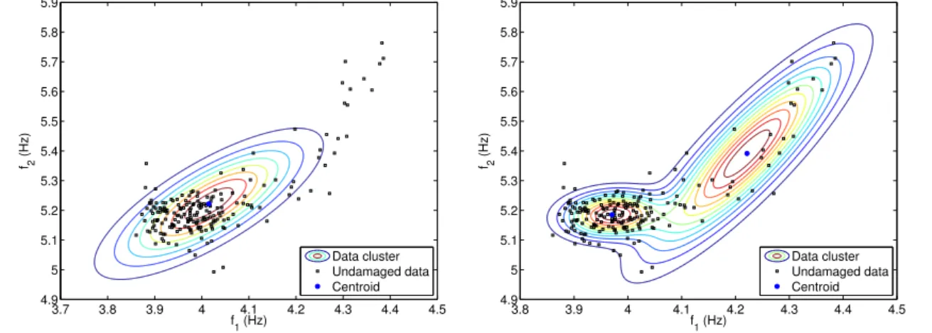
Gaussian mixture models
The penalty term of BIC depends on the size of the training data and is therefore often more severe than that of AIC. The previous chapter was devoted to the description of the SPR paradigm and the main statistical methods for data normalization described in the literature. The breakthrough in this area was achieved by (HINTON; SALAKHUTDINOV, 2006; RANZATO et al., 2007; BENGIO et al., 2007) with the development of a two-phase training program: greedy, layered, unsupervised pretraining followed by supervised focusing.
Autoencoders
This new training program has dramatically improved the performance of such methods, triggering intensive research efforts in the field (ERHAN et al., 2010), especially in the unsupervised sector. In this context, methods based on stacked autoencoders have attracted the most attention in recent years. In this case, an undercomplete autoencoder learns to span the main subspace of the training data, i.e. the same subspace as PCA.
Stacked autoencoders
In the context of SHM, the DSA allows learning more reliable representations of the input vectors as a result of successively applied nonlinear transformations. Here, a nine-layer DSA is trained for SHM to represent, in the bottleneck layer, low-level features from training matrixX. These new features should characterize the hidden factors that changed the underlying distribution of the structural dynamic response.

Deep autoencoders and traditional principal component analysis . 24
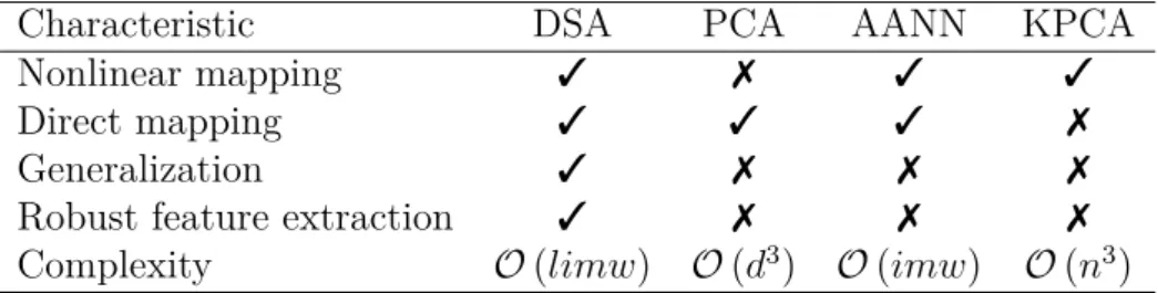
The corresponding computational complexity is therefore determined by the characteristics of the data set such as the number of samples and their dimensionality, as well as the input parameters of each algorithm, such as the target dimensionality 𝑑 and the number of iterations𝑖 (for iterative techniques). In the case of neural networks, 𝑤 denotes the size of the model by the number of weights and 𝑙 the number of layers. From the discussion of the five general properties above it is possible to derive some considerations: (1) some techniques do not provide a direct mapping between the original space and the mapped one, (2) when the number of factors that to be retained is close to the number of samples, 𝑑 ≈ 𝑛, nonlinear techniques have computational disadvantages compared to linear PCA, and (3) a significant number of nonlinear techniques suffer from high demands of computational effort.
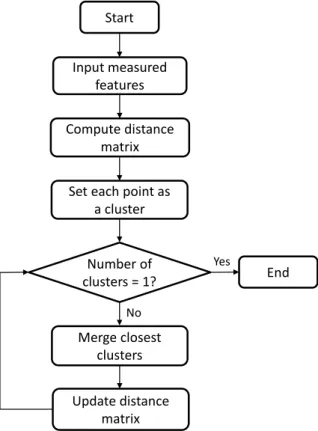
Agglomerative concentric hyperspheres
- Initialization procedures
Note that the main goal of the clustering step is to maximize the observation density associated with each cluster. The convergence is guaranteed by gradual decrease in the observation density as the hypersphere continues to inflate. Each new point is split into other two points in opposite directions placed around dense regions of the feature space.

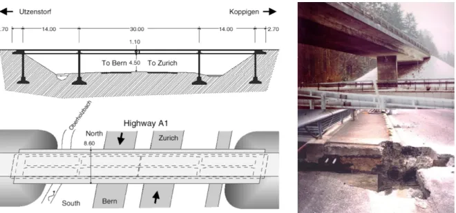
Z-24 Bridge data sets
In this case, the natural frequencies of the Z-24 bridge are used as damage-sensitive functions. Note that the damage scenarios are executed sequentially, resulting in a cumulative degradation of the bridge. The remaining 10% of the characteristic vectors are used during the test phase to ensure that DIs are not triggered before the damage starts.
Tamar Bridge data sets
The data collected in the period from July 1, 2007 to February 24, 2009 (602 observations) were then transferred directly to the computer system and eigenfrequencies were estimated using the stochastic subspace identification technique based on reference data (PEETERS, 1999). From the total number of 602 observations, the first 363 are used for statistical modeling in the training process (corresponding to a one-year follow-up from July 1, 2007 to June 30, 2008), and the entire data sets are used in the testing process, yielding the training matrix X observations) and the test matrix Z of observations). Observations in the interval 1–363 are used in statistical modeling, while observations 364–602 are only used in the test phase (FIGUEIREDO et al., 2012).

Parameter tuning
PCA-based approaches
For evaluation of the DSA-based approach with PCA-based approaches, the number of Type I and Type II errors for the test matrix is presented in Table 3 . Considering a significance level of 5%, the DSA algorithm has the lesser amount of false alarms (even more than the KPCA-based approach). Specifically, the DSA was able to provide the best performance in terms of normalizing the normal variations with a number of type I errors less than 5% of the total uncorrupted data.
Comparative study of the initialization procedures
Basically, the uniform initialization demonstrates a high degree of generalization and robustness to fit the normal state at the expense of losing sensitivity to detect anomalies, as given by a large number of Type II errors (19). On the other hand, the divisive initialization establishes a trade-off between generalization and sensitivity, reaching a low number of Type II errors (6) and maintaining an acceptable number of Type I errors (188), indicating effectiveness to model the normal state and to overcome the non-linear effects. In terms of the number of data clusters, ACH was able to find six, five, and three clusters when paired with uniform, random, and divisive initializations, respectively.

Cluster-based approaches
Basically, for a level of significance around 5%, the ACH provides the best results in terms of total number of misclassifications, less than 5% of the total test data. The ACH yields a monotonic relationship in the amplitude of the DIs related to the damage level accumulation, while the GMM fails to establish this relationship. However, the ACH achieves the best results with only three clusters (𝐾 = 3), indicating that the GMM has generalization problems, which can be explained by a tendency of overfitting caused by a large number of clusters.

Damage detection with daily data set from the Tamar Bridge
PCA-based approaches
On the other hand, the DSA, PCA and AANN based approaches seem to yield a random pattern among the expected outlier observations, especially among those not used in the training process, indicating that the normal state is well understood by the defined models . by both algorithms. Note that in this case there is no evidence of the existence of either damage or extreme operational and environmental variability in the data set. Moreover, the importance of this result is rooted in the fact that this scenario is close to those found in real-world monitoring, where there are no indications of damage a priori, which makes it possible to reduce the number of false alarms and increase the chance. reliability of the SHM system.
Cluster-based approaches
This indicates that the linear behavior of the structure makes it possible to model its normal state using only linear approximations. It shows that for the GMM-based approach, a concentration of outliers is observed in the data not used in the training phase, suggesting an inappropriate modeling of the normal state. On the other hand, the ACH-based approach seems to produce a random pattern among the expected outlier observations, especially among those not used in training process, suggesting a proper understanding of the normal state through the unique clustering that occurs over the training data is defined.
Overall analysis
This new agglomerative concentric hypersphere (ACH) algorithm evaluates the spatial geometry and pattern density of each cluster and can be a significant advance towards cluster-based methods as it requires no input parameters (except the learning matrix) and eliminates the need for resource-related measures variability. Although DSA provides the most robust model, ACH has the advantage of providing a model capable of performing physical interpretations related to sources of variability that alter structural responses (i.e., each cluster may be associated with a different source of variability changing structural properties over a given period ). In this context, DSA provides a black box model that does not provide physical meanings, nor does it contribute to increasing knowledge related to the nature and behavior of the structure.

Future research topics
In terms of overall analysis, as verified on the testbed structures, the proposed approaches demonstrate that they are: (i) as robust as their respective traditional approaches to detect the existence of damage; and (ii) potentially more effective at modeling the baseline and removing the effects of operational and environmental variability, as suggested by minimizing misclassifications of the data from both structures. Moreover, the ACH algorithm also demonstrated high reliability in modeling the normal state and minimizing misclassifications. The ACH thus fits into the category in which results are often acceptable, regardless of the complexity of the structure, with the addendum of providing a model that allows physical interpretation.
Published works
Output-based structural health monitoring based on mean shift clustering for vibration-based damage detection”, 8th European Workshop on Structural Health Monitoring (EWSHM), 2016, Bilbao. Journal of Intelligent Material Systems and Structures, v. Distinguishing between sensor errors, structural damage, and environmental or operational effects in structural health monitoring. Output-only structural health monitoring in changing environmental conditions using nonlinear system identification.