Multi-fidelity Methods for Improved Efficiency in Multi-disciplinary Optimization Problems

Então, a extensão dos esquemas de transferência é aplicada a um problema SEGO utilizando a melhor abordagem. Em seguida, a extensão dos esquemas de transferência é aplicada na melhor abordagem ao SEGO multifidelidade para o mesmo problema.

Nomenclature

Acronyms

Introduction

• Motivation
• Topic Overview
• Surrogate Models
• Bayesian Optimization
• Aircraft Design
• Fluid-Structure Interaction
• Objectives and Deliverables
• Thesis Outline

Aerospace engineering, due to its complexity and multi-disciplinary nature, was one of the first applications of MDO. Extending multidisciplinary optimization to multi-fidelity Figure 1.6: Simplified schematic of the two main topics of the thesis.

Surrogate Modeling and Bayesian Optimization

Multiple Information Source Surrogate Modeling

• Design of Experiments
• Surrogate Modeling via Kriging
• Multi-fidelity Kriging
• Kriging Model combined with Partial Least Squares

The kriging model assumes that the approximation of the outcome of interest(x) takes the form ˆ. One of the most commonly used kernels in kriging is the squared exponential correlation kernel.

Bayesian Optimization

• Efficient Global Optimization (EGO)
• Super-Efficient Global Optimization (SEGO)
• Multi-fidelity Super-Efficient Global Optimization (MFSEGO)

Equation (2.25) is a balance between searching for promising areas of the design space (exploration) and choosing something from where we can learn the design space better (exploration). The choice of the next sample is driven only by the W B2 of the objective function. Then the surrogate model is built based on this DOE and the maximization of the ISC is calculated to obtain the next sample to add to the dataset.

Then, the next high fidelity sample added in the fourth iteration finds the global optimum for the function. The enrichment level, where the algorithm calculates the answer yn+1 for the next sample to be added to the data set, is more complex and is schematized below in Figure 2.10 (b).

Surrogate Modeling Toolboxes

The surrogate model is then reconstructed using the additional information added to the database. It includes the kriging model using the partial least squares approach for single and multiple fidelity (KPLS, MKPLS) [42]. An example of how to use the SMT package to build a kriging model is shown in the Python script below.

The DOE to train the model is defined in xt and yt vectors and the theta is set to 1×10−2. Although the SBS library includes the EGO implementation, the updated EGO for constraints (SEGO) implementation for single and multi-fidelity is a confidential Python package developed by ONERA.

Multi-disciplinary Design Analysis and Optimization

• Terminology and Mathematical Notation
• Architectures
• Multi-Disciplinary Analysis (MDA)
• Gauss-Seidel and Newton MDA
• Aerodynamics and Structures MDA
• Optimization Methods and Sensitivity Analysis
• Gradient-free Methods
• Gradient-based Methods
• Sensitivity analysis
• Discipline Models
• Aerodynamics
• Structures
• Fluid-structure Interaction

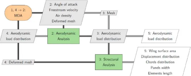
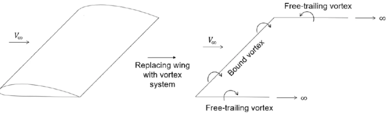
Different approaches can be used to solve the governing equations of discipline analyses, the inner loop in Figure 3.1. This method is used to calculate the derivatives when maximizing the fill sampling criterion W B2 using the SLSQP algorithm. Analyzing Figure 3.8, we notice that only a single bound vortex of power Γ1 acts on the entire span of the wing from point to point b.

In the previous section we have established how we can determine the aerodynamic effect of the lifting surface. As discussed in the previous section, the aerodynamic analysis provides a set of loads applied to each of the aerodynamic panels.

Aero-Structural Design Analysis and Optimization Framework

• Aero-structural Design and Optimization Tool
• Aerodynamic Mesh and Finite Element Structure
• Load and Displacement Transfer Schemes
• Consistency and Conservation Requirements
• Implemented Scheme
• Transfer Schemes for Non-identical Discipline Discretization
• Load Transfer
• Displacement Transfer

As an example of mesh generation, Figure 4.1 shows an aerodynamic mesh constructed from the CRM shape. In addition, figure 4.3 illustrates an aerodynamic panelABCD, the two spanwise (y) aligned structural nodes1 and 2, the position vectors from the structural nodes to the center of the panel of pressurecp(rcp,1, rcp,2) and the forces and moments that have been transferred to them (Fs,1,Fs,2, Ms,1, Ms,2). As observed in Figure 4.3, the load distribution is applied to cp, which is located at the center of the panel ABCDi in the spanwise direction (y), so that half of Ti is applied to each of the structural nodes1and2.

The position vectors are defined from the center of the structural beam element to the panel's center of pressurecp, so instead of each panel having two position vectors, as illustrated in figure 4.3, it has only one, as illustrated in figure 4.9. For figure 4.6 (a) the Aerodynamic Discretization (AD) is more refined than Structural Discretization (SD) and for figure 4.6 (b) SD is more refined than AD.

Comparison of Optimization using Different Multi-fidelity Levels

Optimization Problem Definition

The design variables wing twist and spar thickness are implemented by a spline spanwise distribution. We set the number of control points for these design variables and define a b-spline curve from them. To ensure the non-failure of all finite elements, a von-Mises yield criterion evaluates the structural integrity.

The yield strength of the rod material is represented by σy and a safety factor of 2.5 is used. We use a constraint clustering method based on the Kreisselmeier-Steinhauser function [59], so instead of defining a constraint for each flap element, a single error constraint must be used.

Constants and Optimizer Parameters

In the exponent, R is the range, CT is the specific fuel consumption, CL is the coefficient of lift, V is the airspeed and CD. The last row of Table 5.4 is the relative tolerance used for the convergence of the optimization problem when using the SLSQP optimizer.

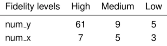
Fidelity Levels and Associated Cost

The discretization associated with each fidelity level is summarized in Table 5.5 and it is illustrated in Figure 5.2 (a), (b) and (c). In industrial problems, the cost ratios imposed on a sample of each fidelity level are linked to the computational time needed to run the analysis. As we test an optimization algorithm, we impose the cost at each fidelity level to be more related to real problems.

The cost ratios established for a sample of each fidelity level are summarized in Table 5.6. Loyalty cost High Medium Low Normalized cost Table 5.6: Cost ratios associated with each level of loyalty.

Design of Experiments Sampling Size

Correlation between Fidelity Levels

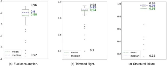
The Pearson coefficient is measured between high fidelity and medium fidelity and high fidelity and low fidelity samples for the objective function and the two constraint functions of the optimization problem, defined in table 5.1. Examining figure 5.3, we observe that the majority of the high-fidelity and medium-fidelity samples have a Pearson coefficient close to one, that is, these samples have a strong positive linear relationship. Thus, one can conclude that the medium fidelity samples add valuable information to the model.

Thus, we conclude that the quality of information provided by samples with low fidelity to the model is highly dependent on the DOE. This figure illustrates the previous conclusions, as we observe stronger linear correlation between high and medium reliability samples than between high and low reliability samples.

Multi-fidelity Parameters Definition

In statistical analysis, the p-value is a number between zero and one that represents the probability of obtaining test results at least as extreme as the actually observed results, assuming that the null hypothesis is correct [62]. If the p-value is less than the threshold, the null hypothesis can be rejected. It is important to note that this budget is only for the optimization process and does not include the costs associated with each DOE presented in Table 5.8.

The optimizer used to maximize the WB2 criterion at each iteration step is SLSQP. The root mean square constraint violation (RSCV) is used to evaluate the results in terms of constraint violation and is given by.

Comparison of Different Multi-fidelity Levels in Optimization

• Reference Solution
• One Fidelity Level Optimization
• Two Fidelity Levels Optimization
• Three Fidelity Levels Optimization

Therefore, the fuel consumption values ​​of the 2 F modified DOE solutions have a tendency to be lower than those of 2 F complete DOE. Then we draw figure 5.11 (a), (b), (c) and (d) which associates the fuel consumption and the log (RSCV) value of the best solution with the number of samples queried per fidelity. Examining figure 5.11, we observe that the maximum values ​​of the fuel consumption for the full DOE approach are greater than the modified DOE, for the same number of query HF samples (110, 109 and 108).

The DOE of the modified DOE has less 120 LF and 40 Medium Fidelity (MF) samples than the full DOE. The optimizations that met the requirements of the full DOE approach tend to choose the number of HF samples between [40, 59], while those of the modified DOE tend to choose the number of HF samples between [60, 78] to choose.

Optimization using Two Multi-fidelity Levels for Non-identical Discipline DiscretizationDiscipline Discretization

The number of acceptable driving tests was 86, which is a significant increase compared to the number of acceptable driving tests of the 2 F approach in Table 5.12.

Summary and Overview

Conclusions

Summary and Achievements

Future Work

After this update, a conservation study of the aerodynamic and structural virtual work should be performed using load transfer method one and two and the displacement transfer. From this study it can be deduced which of the proposal methods has a better performance in terms of virtual work preservation. Then more detailed mesh convergence studies with non-identical discipline meshes can be done and multi-fidelity SEGO using the new updated OAS capability can be performed.

Another interesting development would be to implement the derivatives on the new transfer schemes and all the functions created in OAS in order to enable different discipline discretizations. In this way, the transfer schemes can be updated in the OAS Github repository and problems using gradient-based optimizer with different discipline discretizations can be run.

Bibliography

A comparison of three methods for selecting values ​​of input variables in the analysis of output from a computer code. Global versus local search in constrained optimization of computer models.Lecture Notes-Monograph Series, pages. Extensions to the design structure matrix for describing multidisciplinary design, analysis and optimization processes. Structural and Multidisciplinary Optimization.

The use of the construction structure matrix in system decomposition and integration problems: a review and new directions. Review and unification of methods for calculating derivatives of multidisciplinary computer models. AIAA Magazine.

Appendix A

• Aero-Structural Design and Optimization Tool: OpenAeroStruct
• Mesh Convergence for Identical Spanwise Discipline Discretiza- tiontion
• Correlation between Three Fidelity levels Modified DOE
• Optimization History of the 59 th Acceptable Run Test of the Optimization for Two Fidelity Levels using Modified DOEOptimization for Two Fidelity Levels using Modified DOE
• Mesh Convergence for Non-identical Spanwise Discipline Dis- cretizationcretization
• Fuel Consumption
• Trimmed Flight
• Structural Failure
• Computational Time
• Conclusion
• Optimization using Different Multi-fidelity Levels for Non-identical Discipline DiscretizationDiscipline Discretization
• Correlation between Fidelity Levels
• Scatter Plot
• Solutions of the gradient-based and gradient-free approaches
• Reference Solution
• Solution for the Optimization with Two Fidelity Levels using Modified DOE
• Solution for the Optimization with Two Fidelity Level using Modified DOE and Non-identical Discipline Discretizationand Non-identical Discipline Discretization

When the SD is coarse, as in the example illustrated in figure A.7, fewer elements discretize the wing spar. The structural mass increases dramatically when the SD is coarse, as can be observed in figure A.6 (a) in the three rightmost columns. Examining the lift coefficient histogram in figure A.9 (b), we observe that for the same AD the CL.

Starting with the analysis of Figure A.11 (a), we note that when AD is constant and SD decreases, the tip displacement increases and deviates from the most accurate value (far left column). In Figure A.15, we notice that the buoyancy distribution of the reference solution is not elliptical.