PDF DOE - pedro.unifei.edu.br

DOE

Design of Experiments / Factorial / Fractional / RSM

UNIFEI Jul 2017

Six Sigma | P. P. Balestrassi

2

Temperatura

170,0 167,5 165,0 162,5 160,0

Rendimento

42 69 71 Viscosidade 38

Overlaid Contour Plot of Rendimento; Viscosidade

An overview of

Design of Experiments

Summary

• Efficient Experimentation

• Factorial Designs

• Fractional Factorial Designs

• Screening Designs

• Taguchi Designs

• Response Surface Methodology

• Desirability

• Mixtures

Pedro P. Balestrassi

“Statistical thinking will one day be as necessary for

efficient citizenship as the ability to read and write.”

H. G. Wells (Writer, 1895)

ra

170,0 167,5

Rendimento

42 69 71 Viscosidade 38

Overlaid Contour Plot of Rendimento; Viscosidade

Statistical thinking Introduction

Factors of a Process

Process

Noise Factors Control Factors

Input Output

...

x ¹ x ² ... x ^p

z ¹ z ² z ^q

y ¹ y ² y ^m

... Source Client

SIPOC

Efficient

Experimentation

Robust Process

• Which factors influence y ^the

most?

• How to adjust x to get the desired value for y ^?

• How to adjust x to achieve minimal variation for y ^?

• How to adjust x so that the

z y

What is

Robustness?

Efficient

Experimentation

X

• Air strip pressure

• Air bag pressure

• Air front piston pressure

• Hydraulic pressure

• Temperature

• Oil flow

• Nitrogen pressure

Y

• Top Wall width

• Mid Wall width

• Dome depth

• Can height

• Painting

Bodymaker Process

Z

• Operator

• Electricity fluctuation

• Aluminiun quality

Example: Can Making

It’s complicated to infer about X,Y and Z without statistics

Y=f(X)+Z+e

Efficient

Experimentation

X

• Injection time

• Cooling time

• Mold temperature

• Machine temperature

• Injection velocity

• Injection pressure

Y

• Scrap

• Deformation

• Failure rate

Example: Injection Molding

Z

• Cycle time

• Operator

• ...

Efficient

Experimentation

TRIP Process of Can Making

- Ph da pré-lavagem

- Temperatura da lavagem química - Acidez livre da lavagem química - Acidez total da lavagem química - Milivolt da lavagem química - Ph do tratamento

- Temperatura do tratamento - Milivolt do tratamento - Teor de sílica

- Teor de cloro do mobility

- Pressão de vácuo da roda de transferência - Velocidade da printer

- Condutibilidade do mobility - Concentração do mobility

- Temperatura da primeira zona do forno - Temperatura da segunda zona do forno - Velocidade da lavadora

- Pressão superior do spray na pré-lavagem - Pressão inferior do spray na pré-lavagem - Pressão superior do spray na lavagem química - Pressão inferior do spray na lavagem química - Pressão superior do spray no tratamento - Pressão superior do spray no mobility - Pressão inferior do spray no mobility

- Condição da esteira de aço - Condição da esteira plástica da lavagem

- Qualidade do produto

- Condição do punção da bodymaker - Fundo fraturado

- Sujeira no conveyor - Desgaste do assento azul

- Lata chaleira

- Lata com rugas no fundo - Lata com rebarba

- Lata ovalizada

- Sujeira na calha de alimentação da printer

- Sincronismo da roda de transferência

- Sujeira no mandril - Mangueiras estouradas - Desgaste do wiper - Sujeira no single filer - Sujeira nos assentos azuis - Ajuste do manifold

7 Outputs -

Can features after TRIP process.

- Latas cortadas impregnadas de óleo solúvel - Ácido sulfúrico - Ridoline 1895 - Ridoline 120 - Alodine 404NC - Mobility ME 60 - Gás

- Dicloro

- Água deionizada

CONTROL

NOISE

Input

→

Z X

Y

How to handle this type of problem?

24 Factors

18 Factors

9

Inputs

Efficient

Experimentation

Experiment X1 X2 X3 X4 X5 X6 X7 Results

1. – – – – – – – 2.1

2. + – – – – – – 2.6

3. + + – – – – – 2.4

4. + – + – – – – 2.5

5. + – – + – – – 2.8

6. + – – + + – – 2.9

7. + – – + + + – 2.7

8. + – – + + – + 3.2

Final + – – + + – +

Consider the experimental design in 2-levels (-/+) for the factors X1 .. X7

Stick-a-winner Strategy ^Efficient

Experimentation

Experiment X1 X2 X3 X4 X5 X6 X7 Results

1. – – – – – – – 2.1

2. + – – – – – – 2.5

3. – + – – – – – 1.9

4. – – + – – – – 1.9

5. – – – + – – – 2.2

6. – – – – + – – 2.3

7. – – – – – + – 2.5

8. – – – – – – + 2.3

Final + – – + + + +

Another Common Sense approach

Consider the experimental design in 2-levels (-/+) for the factors X1 .. X7

The Stick-a-winner Strategy is a One-factor-at-a-time method to run experiments.

Efficient

Experimentation

• These methods are conventional (common sense).

• These methods are inefficient in determining the main factors.

• Interaction is totally negleted in this type of method.

One-factor-at-a-time method ^Efficient

Experimentation

Health

Alcohol

Without Good

With Regular

Excelent

Death

Interaction

With Medicine Without Medicine

Efficient

Experimentation

DOE for practitioners

• Knowledge of specialist is fundamental;

• DOE means simplicity;

• DOE recognizes what is important;

• Experiments are interactive

One-factor-at-a-time (Common Sense)

Factors vary simultaneously

(Central idea on DOE) X

Efficient

Experimentation

• Assume that you work at a chemical plant.

• You are studying one of the reactions that produces a chemical product.

• You would like to somehow increase the yield of a product that is produced by the reaction.

• From past experience, you have seen that varying the temperature, the pressure, and the type of catalyst seem to change the yield of the reaction.

• The problem is that everyone you work with has their own theory about how each of these factors affects the reaction.

• You want to make real improvements, so you decide to run an experiment to determine the actual effects of these three factors:

1. Temperature (Levels of 40 ^o C and 60 ^o C) 2. Catalyst (Levels A and B)

3. Pressure (Levels of 1 and 1.5 atmospheres)

An example of DOE using Minitab ^Efficient

Experimentation

Minitab Worksheet

2 ³

Full Factorial Design with 2 Replicates

Efficient

Experimentation

P_value <0.05 → Coefficient is significant.

DOE Results

Factorial Fit: Yield (grams) versus Temperature, Catalyst, Pressure Estimated Effects and Coefficients for Yield (grams) (coded units)

Term effect Coef SE T P Constant 74.75 2.543 29.39 0.000 Temperature 1.25 0.63 2.543 0.25 0.812 Catalyst 14.00 7.00 2.543 2.75 0.025 Pressure -30.50 -15.25 2.543 -6.00 0.000 Temperature*Catalyst -0.25 -0.12 2.543 -0.05 0.962 Temperature*Pressure -1.25 -0.63 2.543 -0.25 0.812 Catalyst*Pressure -13.50 -6.75 2.543 -2.65 0.029 Temperature*Catalyst*Pressure -0.25 -0.13 2.543 -0.05 0.962

Efficient

Experimentation

Pareto Chart

Te rm

AB ABC A AC BC B C

6 5

4 3

2 1

0

2.306

F actor Name A Temperature B C ataly st C Pressure

Pareto Chart of the Standardized Effects

(response is Yield (grams), Alpha = .05)

Efficient

Experimentation

Normal Plot

Standardized Effect

P e rc e n t

3 2

1 0

-1 -2

-3 -4

-5 -6

99

95 90 80 70 60 50 40 30 20 10 5

1

F actor Name A Temperature B C ataly st C Pressure Effect Type Not Significant Significant

BC

C

B

Normal Probability Plot of the Standardized Effects

(response is Yield (grams), Alpha = .05)

Efficient

Experimentation

Factorial Plots

M e a n o f Y ie ld ( g ra m s)

60 40

90 80 70

60

B A

90 80 70 60

Temperature Catalyst

Pressure

Main Effects Plot (data means) for Yield (grams)

Efficient

Experimentation

T emperature

B

A 1.0 1.5

100

80

60

Catalyst

100

80

60

Pr essur e

Temperature 40 60

Catalyst A B

Interaction Plot (data means) for Yield (grams)

There is an interaction between Pressure and Catalyst that effects the Response.

Interaction ^Efficient

Experimentation

1.5

1 B

A

Pressure Catalyst

59.5

59.5 59.0

60.0

105.0

77.5 75.0

102.5

Cube Plot (data means) for Yield (grams)

The Cube Plot represents the experimental space at two levels. Axial values are the average of the replicates.

Cube Plot ^Efficient

Experimentation

Thinking Ahead ...

Process

Noise Factors Control Factors

Input Output

...

x ¹ x ² ... x ^p

z ¹ z ² z ^q

y ¹ y ² y ^m

... Source Client

Efficient

Experimentation

Design of Experiments

Renaissance of DOE in industry:

• Efficient computational softwares (JMP, Statistica, Minitab, WebDOE, SPSS, etc...)

• Six Sigma Methodology

✓Determining the main factors in a process (Screening DOE)

✓Establishing transfer function and optimization.

(Factorial DOE and RSM)

Y=f(X) +Z +e

Efficient

Experimentation

• ... a technique to decrease the amount of experiments (or

simulation)

• ... a graphical method to analyse experiments

•... a numerical method to analyse experiments

Use DOE as ... ^Efficient

Experimentation

Which combinations are missing?

Factor 1 Run

– + – – 1

2 3 4

– – + –

– – – + Factor

2

Factor 3

5 6 7 8

‘-’ represents the lower level and

‘+’ represents the upper level

Transition to DOE

- + -

- - +

+ - -

- - - 6

3

7 8

4

1 2

5

In the One-factor-at-a-time method the space is not balanced.

Factorial Designs

– + – + – + – + Factor

1 1

2 3 4 5 6 7 8

– – + + – – + +

– – – – + + + + Factor

2

Factor 3

Standard Order

Full Factorial

The Standard Order is not always the Run Order

Factorial Designs

Yellow Green Yellow Green Yellow Green Yellow

Factor 1

1 2 3 4 5 6 7

Standard Order

1.42 1.42 2.00 2.00 1.42 1.42 2.00

3.00 3.00 3.00 3.00 4.75 4.75 4.75 Factor 2 Factor 3

Factors are Qualitative or Quantitative

Full Factorial

2 ³

Factorial Designs

Experimental space

2 Factors = A Square

Factor 1

– +

Factor 2

+

–

Factor 2

Factor 1

– +

+

– –

+

Factor 3 3 Factors = A Cube

Cube Plot Factorial Designs

4 Factors: Two Cubes

– +

Factor 4

Fourth Dimension Factorial Designs

–

Factor D

+

– +

Factor D Factor E

(-)

Factor E (+) A

B

C

1 = - - - - -

16 = ++++- 8 = +++ - -

17 = - - - - +

32 = +++++

5 Factors:

4 Cubes

Cube Plot Factorial Designs

runs = 2 ^k

• The whole experimental space is covered with

Factorial Designs.

• Factorial Designs are easy to conduct due to a well-

established pattern.

DOE Matrix

# of factors

Standard Order

Factorial Designs

Simple Model

Y=Constant + <Average>

k ¹ X1 + k ² X2 +k ³ X3 + <Main Factors >

k ⁴ X1X2 + k ⁵ X1X3 + k ⁶ X2X3 + <2 ^nd Order Interactions>

k ⁷ X1X2X3 <3 ^rd Order Interaction >

Y = f (X ₁ , X ₂ , X ₃ , …, X _n )

Y (Response)

X _i (Factors) = X1, X2, X3

Factorial Designs

Constant

Order Std.

1 2 3 4 5 6 7 8

X1 – + + + + – – –

X2 – – + + – – + +

X3 – – – –

+ + + +

Data

(Rep 1, Rep 2, Rep 3) 49.5

49.5 49.75 48.75 51.25 50.00 49.50 50.50

Average

Sum _______ 1194.50 Average _____ 49.77 50.75

48.75 49.25 48.25 49.75 50.00 50.50 50.50

50.00 49.50 48.50 49.00 50.25 50.75 49.75 50.25

Y=49,77 + k ¹ X1 + k ² X2 +k ³ X3 + k ⁴ X1X2 + k ⁵ X1X3 + k ⁶ X2X3 + k ⁷ X1X2X3

Factorial Designs

Main Effects

Order Std.

1 2 3 4 5 6 7 8

– + + + + – – –

– – + + – – + +

– – – –

+ + + +

Average 50.10 49.25 49.17 48.67 50.42 50.25 50.42 49.92

X3 “+”

50.42 50.25 50.42 49.92 X3 “-”

50.10 49.25 49.17 48.67

Total X3 “+” _____ 201.01 Total X3 “-” _____ 197.19

Average of X3 “-” _____ 49.30

Average of X3 “+” _____ 50.25 Effect of X3 = [Average of X3 “+”] - [ Average of X3 “-”] = 0.95

X1 X2 X3

When X3 goes from “-” to “+” the response Y increases 0.95

Factorial Designs

- +

- +

Y 49 49. 5 50 50. 5

49.77

0 X3

X2

Y 49 49. 5 50 50. 5

When X3 goes from “-” to “+” the response Y increases 0.95

When X2 goes from “-” to “+” the response Y decreases 0.45

Main Effects Factorial Designs

Coefficients

A Effect

2 q

2

Effect tg q = A

Level

-1 +1

Response

29,50 29,75 30,00 30,25 30,50 30,75 31,00

Factor A

Factorial Designs

Coefficient of X3

- +

Y 49 49 .5 50 50 .5

49.77

0 X3

Y=49,77 + k ¹ X1 + k ² X2 +0.497X3 + k ⁴ X1X2 + k ⁵ X1X3 + k ⁶ X2X3 + k ⁷ X1X2X3

When X3 goes from “-” to “+” the response Y increases 0.95

k 3 = 0.95/2

Factorial Designs

Interaction Effect - Example

A B AB Response

- - + 50

+ - - 54

- + - 100

+ + + 60

AB Effect = (Average of AB “+” ) - (Average of AB “-”) AB Effect = (50+60)/2 - (54+100)/2

AB Effect = - 22

Coefficient of AB = - 11

Response= Constant + k

A + k 2 B – 11AB

— Terminology:

A x B or AB

Factorial Designs

Interaction Plot

Response

Factor A

Factor B

+ –

– +

Factor A

Factor B

+ –

– +

+ –

– +

Factor A

Factor B

+ –

– +

+ –

– +

+ –

– +

High Interaction No Interaction

Low Interaction

Evaluate also P_value

ResponseResponse Response

Factor A

Factor B

Factor A

Factor B

Factor A

Factor B

ResponseResponse

Factorial Designs

Design with interactions

Response

________

________

________

________

________

________

________

Std.

Order 1 2 3 4 5 6 7 8

A – + – + – + – +

B – – + + – – + +

C – – – – + + + +

AB + – – + + – – +

AC + – + – – + – +

BC + + – – – – + +

ABC – + + – + – – +

________

2 ³ Factorial Design Not usually visible

Factorial Designs

P-Value / Test of Hipothesys

▪ H _o : factor is in the group

▪ H _a : factor is different from the group

▪ If p < a: H _o is rejected

Factorial Designs

Response= 50+ 0,5A+ 0,3B

Level

(-1) (+1) Factor A 10 20 Factor B 0 10

Max Response= 50+0,5(+1)+0,3(+1)=50,8

Coded Unit Factorial Designs

Example Factorial Designs

Main Effects Factorial Designs

Interaction Plots Factorial Designs

Surface Plots Factorial Designs

Contour Plots Factorial Designs

a) What is the linear model?

b) What is the main factor?

c) Does it have interaction among the factors?

Temperature Catalyst Yield (grams)

Example Factorial Designs

Temperature Catalyst Pressure Yield

Example

a) What is the linear model?

b) What is the main factor?

c) Does it have interaction among the factors?

Factorial Designs

Temperature Catalyst Pressure PH Yield

Example

a) What is the linear model?

b) What is the main factor?

c) Does it have interaction among the factors?

Factorial Designs

Full Factorial problems

Number of Factors

1 2 3 4 5 6 7 8 9 10

•

•

• 15

•

•

•

Number of Experiments

2 4 8 16 32 64 128 256 512 1024

•

•

• 32,768

•

•

•

2 ^k

Number of Experiments

Fractional Factorial

Design

Available Information

2 ^k

The vast majority of processes are dominated by main effects and lower order

interactions

Number of Factors

1 2 3 4 5 6 7 8 9 10

•

•

• 15

•

•

• 20

1 2 3 4 5 6 7 8 9 10

•

•

• 15

•

•

• 20 Main Effects

2

Order Interaction

– 1 3 6 10 15 21 28 36 45

•

•

• 105

•

•

• 190

– – 1 5 16 42 99 219 466 968

•

•

• 32,647

•

•

• 1,048,365

> 2

Order Interaction

Fractional Factorial

Design

Example for 4 factors

2 ⁴

Response=Constant+ <Average>

A B C D + <Main Effects>

AB AC AD BC BD CD + <2

Interactions>

ABC ABD ACD BCD + < 3

Interactions>

ABCD < 4

Interaction>

Fractional Factorial

Design

Fractional Factorial

2 ³

A B

C

7 8

3 4

5 6

1 2

– + – + – + – + A Order

– – + + – – + + B

– – – – + + + + C 1

2 3 4 5 6 7 8

2 ^3-1

Half Fraction

Fractional Factorial

Design

Half Fraction

2 ^3-1

A B

C

7 8

3 4

5 6

1 2

+ – + A

– + – + B

– – + + Order C

2 3 5 8

–

Observe that C=AB

Fractional Factorial

Design

Building Half Fraction

2 ^4-1

A B

– + – + – + – +

– – + + – – + +

– – – – + + + + C

– + + – + – – +

D = ABC

2 ³

Base

D=ABC= Design Generator

– + – + – + – + – + – + – + – + A

– – + + – – + + – – + + – – + + B

– – – – + + + + – – – – + + + + C

– – – – – – – – + + + + + + + + D

+ – – + – + + – – + + – + – – + E

2 ^5-1

2 ⁴

Base

E=ABCD= Design Generator

Fractional Factorial

Design

Full Factorial x Half Fraction ---Trade-Offs

Number of Effects

Effects Average Main

2

order Interactions

Total of Effect

Full Fraction 1

5 10 10 5 1 32

1 5 10

—

—

—

16 Number of

experiments

If you don’t have a reason to believe that higher order

interactions are present, you can choose half fraction.

3

order Interactions 4

order Interactions 5

order Interaction

Fractional Factorial

Design

– – – – + + + +

Factor A 1

2 3 4 5 6 7 8 Run

– – – – + + + + Factor B

130 125 133 130 50 85 79 93

Response

Confounding A=B

The Effects of A and B are confounded.

Fractional Factorial

Design

D=ABC

A B C D AB AC

=

=

=

=

=

=

BCD ACD ABD ABC CD BD –

+ – + – + – + A

– – + + – – + + B

– – – – + + + + C

– + + – + – – + D

+ – – + + – – + AB

+ – – + + – – +

CD From the Base D=ABC

A.D=A.ABC=1.BC=BC

AD.D=A.1=D.BC

Etc...

1

1

Fractional Factorial

Design

D=ABC

– + – + – + – + A

– – + + – – + + B

– – – – + + + + C

– + + – + – – + D

+ – – + + – – + AB

+ – – + + – – + CD

10 20 18 12 12 18 20 10

Response

Effect of AB+CD = (10+12+12+10)/4 – (20+18+18+20)/4

= 11-19= -8

This is not AB effect or CD effect exclusively. Also, it is not possible to divide AB + CD.

Meaning of AB+CD Fractional Factorial

Design

Common Sense X DOE

Consider the experimental design in 2-levels (-/+) for the factors X1 .. X7

Experiment X1 X2 X3 X4 X5 X6 X7

1. – – – – – – –

2. + – – – – – –

3. – + – – – – –

4. – – + – – – –

5. – – – + – – –

6. – – – – + – –

7. – – – – – + –

8. – – – – – – +

The Stick-a-winner Strategy is a One-factor-at-a-time method

Fractional Factorial

Design

Common Sense X DOE

Consider the experimental design in 2-levels (-/+) for the factors X1 .. X7

Experiment X1 X2 X3 X4 X5 X6 X7

1. – – – + + + –

2. + – – – – + +

3. – + – – + – +

4. + + – + – – –

5. – – + + – – +

6. + – + – + – –

7. – + + – – + –

8. + + + + + + +

Resolution III Placket-Burman Design

Fractional Factorial

Design

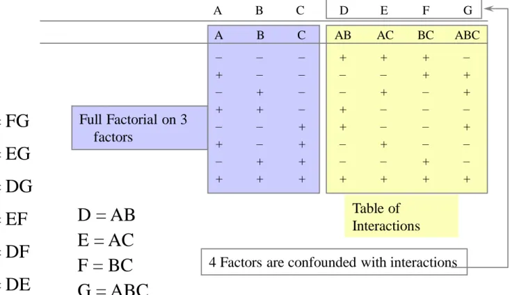
Minimal number of experiments

Ex.: 7 Factors on 8 experiments

Full Factorial on 3 factors

Table of Interactions 4 Factors are confounded with interactions

– + – + – + – +

– – + + – – + +

– – – – + + + +

+ – – + + – – +

+ – + – – + – +

+ + – – – – + +

– + + – + – – +

A B C AB AC BC ABC

A B C D E F G

A B C D E F

=

=

=

=

=

= BD AD AE AB AC AG

CE CF BF CG BG BC

FG EG DG EF DF DE

=

=

=

=

=

=

=

=

=

=

=

=

D = AB E = AC F = BC

Screening Designs Fractional Factorial

Design

Display available design Fractional Factorial

Design

Design’s Resolution

R Confounding III 1-2

IV 1-3 , 2-2 V 1-4 , 2-3

Fractional Factorial

Design

Nomenclature

7 factors 2 levels

Resolution IV

3 main factors confounded with 3 ^rd order interaction

With Replication Total of 32 runs

2 Times

Fractional Factorial

Design

Paper helicopter

(Box, Bisgaard and Fung – Designing

Industrial Experiments: The Engineer’s Key to Quality, 1990)

Fractional Factorial

Design

Resolution III Experiments ^Screening

Design

Example of Screening Design

Objective: Analyze the results of the following factors using Screening Designs.

Data: Damage.mtw

A B C D E F G

Load

Load method Packing

Box size Shipper

Open method

“Use Caution” message on box

partial std.

paper std.

x knife no

full rush

styrofoam custom p

scissors yes

Factors and Levels +

Y = Damage Claim ($)

Background: A mail order company is trying to reduce the Damage Claims caused by boxing, shipping, and opening methods. They ran a design with these factors:

Screening

Design

Session window - Alias ^Screening

Design

Session window - Results

Fractional Factorial Fit

Estimated Effects and Coefficients for $Damage (coded units) Term Effect Coef

Constant 20.375 Load 20.250 10.125 Method 2.250 1.125 Packing 0.750 0.375 Box -2.250 -1.125 Shipper 5.250 2.625 Open -11.750 -5.875 Message -13.250 -6.625

Analysis of Variance for $Damage (coded units)

Source DF Seq SS Adj SS Adj MS F P Main Effects 7 1524 1524 217.7 * * Residual Error 0 0 0 0.0

Total 7 1524

Estimated Coefficients for $Damage using data in uncoded units

Output deleted to save space:same as above for this situation (all factor levels are discrete)

Alias Structure (up to order 3)

I + Load*Method*Box + Load*Packing*Shipper + Load*Open*Message + Method

*Packing*Open + Method*Shipper*Message + Packing*Box*Message + Box*Shipper*Open Load + Method*Box + Packing*Shipper + Open*Message+ Method*Packing*Message + Method*Shipper*Open + Packing*Box*Open + Box*Shipper*Message

Method + Load*Box + Packing*Open + Shipper*Message+ Load*Packing*Message + Load*Shipper*Open + Packing*Box*Shipper + Box*Open*Message

Packing + Load*Shipper + Method*Open + Box*Message+ Load*Method*Message + Load*Box*Open + Method*Box*Shipper + Shipper*Open*Message

Box + Load*Method + Packing*Message + Shipper*Open+ Load*Packing*Open + Load*Shipper*Message + Method*Packing*Shipper + Method*Open*Message Shipper + Load*Packing + Method*Message + Box*Open+ Load*Method*Open + Load*Box*Message + Method*Packing*Box + Packing*Open*Message

Open + Load*Message + Method*Packing + Box*Shipper+ Load*Method*Shipper + Load*Packing*Box + Method*Box*Message + Packing*Shipper*Message

Message + Load*Open + Method*Shipper + Packing*Box+ Load*Method*Packing + Load*Box*Shipper + Method*Box*Open + Packing*Shipper*Open

Coefficients with largest values are highlighted; will need to check plots to see the size relative to each other

since there are no P-values No replicates means no estimate of experimental variability; no t-values; no P-values

Same information here as previous page, but Factor Names used

Screening

Design

Effects plots

• Because there are no replicates and 7 effects estimated in only 8 runs, Minitab cannot produce a P-value reference for these plots.

• It is left to your own judgment to determine which effects seem important enough for you to investigate further.

• 3 effects—load, message, and open—seem relatively larger than the rest

0 10 20

Packing Box Method Shipper Open Message Load

Pareto Chart of the Effects

(response is $Damage, Alpha = .05)

-10 0 10 20

-1.5 -1.0 -0.5 0.0 0.5 1.0 1.5

Effect

Normal Score

Normal Probability Plot of the Effects

(response is $Damage, Alpha = .05)

Screening

Design

Results

• Simplest explanation for three important effects

– Observed results could be due solely to main effects from 3 factors

Load (= A) Open-method (= F) Message-on-box (= G)

• Alternative explanations

– Observed results could also be due to two main effects and their interaction.

If you look carefully at the alias structure, you’ll see that the two-factor interactions of these three factors are confounded with each other as follow:

Screening

Design

Alias Information for Terms in the Model.

Totally confounded terms were removed from the analysis.

•Load + Method*Box + Packing*Shipper + Open*Message

•Method + Load*Box + Packing*Open + Shipper*Message

•Packing + Load*Shipper + Method*Open + Box*Message

•Box + Load*Method + Packing*Message + Shipper*Open

•Shipper + Load*Packing + Method*Message + Box*Open

•Open + Load*Message + Method*Packing + Box*Shipper

•Message + Load*Open + Method*Shipper + Packing*Box

Terms in bold are responsible for 90% of the effects.

Adjusts ^Screening

Design

• Full Factorial Designs can be constructed for any number of factors with any number of

levels. When there are more than two levels, they provide all the benefits of the Factorial designs, as well as the Response Surface

Designs.

1 factor of 2 levels 1 factor of 3 levels

1 factor of 5 levels

Runs=30

Mixed Levels ^Screening

Design

Background: An experiment was desired on finishing a

mechanical device. Response variable was the consistency of lubrication, measured subjectively on a 1–5 scale.

Factors Levels

Precoat Yes

No

Pressure Dies 2% larger than incoming wire 4%

5%

7%

9%

Speed 150 fpm

175 200 225 250 275 300

Example

Data: wire.mtw

Screening

Design

General Linear Model

Factor Type Levels Values Precoat fixed 2 Yes No Pressure fixed 5 2 4 5 7 9

Speed fixed 7 150 175 200 225 250 275 300

Analysis of Variance for Lubricat, using Adjusted SS for Tests Source DF Seq SS Adj SS Adj MS F P Precoat 1 4.129 4.129 4.129 12.80 0.001 Pressure 4 196.057 196.057 49.014 151.91 0.000 Speed 6 2.943 2.943 0.490 1.52 0.188 Error 58 18.714 18.714 0.323

Total 69 221.843

Unusual Observations for Lubricat

Obs Lubricat Fit StDev Fit Residual St Resid 1 3.00000 1.70000 0.23519 1.30000 2.51R 9 4.00000 5.27143 0.23519 -1.27143 -2.46R 47 1.00000 3.04286 0.23519 -2.04286 -3.95R 58 3.00000 1.70000 0.23519 1.30000 2.51R

The effects of Precoat and Pressure are significant.

Speed is borderline.

Example ^Screening

Design

Precoat Pressure Die Speed

1 2 3 4 5

Lubrication

From the graph you can understand the nature of the effects for the factors. From these plots it is easy to see that the 7%

or 9% Pressure Die is much preferred. With these Dies, the Speed and Precoat seems to have minimal effect.

Example ^Screening

Design

1 3 5 1 3 Precoat 5

Pressure Die

Speed Yes

No

2 4 5 7 9

Inte ra c ti o n P lo t - D a ta M e a ns fo r L ub ri c a tio n

Example ^Screening

Design

Research on DOE for Simulation ^Screening

Design

Research on DOE for Simulation ^Screening

Design

Kleijnen

1 2 3 4 5 6 7 8 1 1 1 2 2 2 2 2 A 1 1 2 1 1 2 2 2 B 1 1 2 2 2 1 1 2 C A B C D R1 R2 R3 R4 R5 R6 R7 R8

1 1 1 1 1 16 10 17 20 20 20 20 19 2 1 2 2 2 15 16 19 19 20 20 24 22 3 1 3 3 3 16 17 19 16 23 18 23 20 4 2 1 2 3 18 17 19 19 21 19 23 25 5 2 2 3 1 20 19 19 25 26 21 28 25 6 2 3 1 2 16 16 20 20 15 20 23 25 7 3 1 3 2 16 19 18 24 17 19 24 22 8 3 2 1 3 14 16 15 17 18 20 23 24 9 3 3 2 1 16 20 19 17 23 23 23 29

L ⁹

L ⁸

Crossed Array

Response Outer Array

Inner Array Ex.

Ex.

Control

Noise

Taguchi

Designs

Display available design ^Taguchi

Designs

• Kuerten’s coach used Taguchi Design to improve the serve of Gustavo Kuerten, the best Brazilian tennis player.

Example: Gustavo Kuerten

Level 1 Level 2 Level 3 A Force Low Medium High

B Technique Flat Topspin Slice-Topspin C Frequency

D Racquet Quantun Yonex Wilson Factors

Level 1 Level 2

A Hour Day Night

B Court Clay Grass

C Side Right Left

Factors

Taguchi Designs

Low Medium High

• Taguchi L ₉ Design

• 4 Control Factors in 3 levels

Taguchi Design ^Taguchi

Designs

Force Technique Frequency Racquet

A B C D

Outer Array ^Taguchi

Designs

• Taguchi L ₈ Design

• 3 Noise Factors in 2 levels

Time Court Side

A B C

1 2 3 4 5 6 7 8 1 1 1 2 2 2 2 2 A 1 1 2 1 1 2 2 2 B 1 1 2 2 2 1 1 2 C A B C D R1 R2 R3 R4 R5 R6 R7 R8

1 1 1 1 1 16 10 17 20 20 20 20 19 2 1 2 2 2 15 16 19 19 20 20 24 22 3 1 3 3 3 16 17 19 16 23 18 23 20 4 2 1 2 3 18 17 19 19 21 19 23 25 5 2 2 3 1 20 19 19 25 26 21 28 25 6 2 3 1 2 16 16 20 20 15 20 23 25 7 3 1 3 2 16 19 18 24 17 19 24 22 8 3 2 1 3 14 16 15 17 18 20 23 24

L ⁹

L ⁸

Crossed Array

Outer Array

Inner Array guga.mtw

Taguchi Designs

Smaller is better:

Response is the distance between where the ball hit the court and a

specified target.

Mean of SN ratios

3 2

1 -25.50

-25.75 -26.00 -26.25 -26.50

3 2

1

3 2

1 -25.50

-25.75 -26.00 -26.25 -26.50

3 2

1

Force Technique

Frequency Racquet

Main Effects Plot (data means) for SN ratios

Signal-to-noise: Smaller is better

S/N

Signal/noise ^Taguchi

Designs

 

 



− 

=

 

= n

1 i

2 i

10 y

n log 1

10

Response Table for Signal to Noise Ratios Smaller is better

Level A: Force B: Technique C:Frequency D:Racquet 1 -25.54 -25.78 -25.48 -26.37 2 -26.43 -26.18 -26.22 -25.92 3 -26.06 -26.07 -26.33 -25.74 Delta 0.89 0.40 0.85 0.62 Rank 1 4 2 3

Factor that affect the

S/N - Levels ^Taguchi

Designs

 

 



− 

=

 

= n

1 i

2 i

10 y

n log 1

10

Mean of Means

3 2

1 20.5

20.0 19.5 19.0 18.5

3 2

1

3 2

1 20.5

20.0 19.5 19.0 18.5

3 2

1

Force Technique

Frequency Racquet

Main Effects Plot (data means) for Means

Smaller is better Mean

Target ^Taguchi

Designs

Response Table for Means

Level A: Force B: Technique C:Frequency D:Racquet 1 18.71 19.25 18.50 20.63 2 20.79 20.21 20.25 19.54 3 19.83 19.88 20.58 19.17 Delta 2.08 0.96 2.08 1.46 Rank 1 4 2 3

Main factor

Smaller is Better ^Taguchi

Designs

Order of the Main factors

(1) Force (2) Frequency (3) Racquet (4) Technique

Selected Levels ^Taguchi

Designs

Level 1 Level 2 Level 3 A Force Low Medium High

B Technique Flat Topspin Slice-Topspin C Frequency Low Medium High

D Racquet Quantun Yonex Wilson

Factors

Orthogonal

Array (Sum=0)

Saturated Designs

(Each column one factor)

Array ^Taguchi

Designs

Taguchi Equations ^Taguchi

Designs

16 18 20 22 24 26

42 52 62

7 8 9

Soak Time (min.)

Concentration (%)

Contour Plot of Plating

• Response Surface Methodology refers to the design and analysis of experiments that can model curved relationships. For Response Surface Analysis, all X’s must be continuous variables.

15

Plating (mm)20 25

9.5

x2

x1

y

y

= Plating (mm)

Wire Diagram

What is RSM?

y = f(x ₁ , x ₂ ⁾

RSM

Rotation

Time

3000 2500 2000 1500 1000 130 120 110 100 90 80 70 60 50

C.V. (%) 6 - 8 8 - 10 10 - 12

> 12

< 4 4 - 6 Contour Plot of C.V. (%)

RSM with Minitab RSM

Rotation

Time

3000 2500 2000 1500 1000 130 120 110 100 90 80 70 60 50

C.V. (%) 6 - 8 8 - 10 10 - 12

> 12

< 4 4 - 6 Contour Plot of C.V. (%)

Process Knowledge RSM

Rotation

Time

3000 2500 2000 1500 1000 130 120 110 100 90 80 70 60 50

C.V. (%) 6 - 8 8 - 10 10 - 12

> 12

< 4 4 - 6 Contour Plot of C.V. (%)

• Response Surface Methodology fits these curved surfaces using a quadratic model. A quadratic model in one X has the form:

• Some shapes produced by this model are:

The Quadratic Model, One X

x b x

b a

y = + ₁ + ₂ ²

y y y y

Parabolas RSM

Rotation

Time

3000 2500 2000 1500 1000 130 120 110 100 90 80 70 60 50

C.V. (%) 6 - 8 8 - 10 10 - 12

> 12

< 4 4 - 6 Contour Plot of C.V. (%)

Similarly, a quadratic model for 2 X factors has the form:

The Quadratic Model, Two Xs

x x b x

b x

b x

b x

b a

y = + _{1 1} + _{2 1} ² + _{3 2} + ₄ ² ₂ + _{5 1 2}

Peak or Valley Rising RidgeRising Ridge

RSM

Rotation

Time

3000 2500 2000 1500 1000 130 120 110 100 90 80 70 60 50

C.V. (%) 6 - 8 8 - 10 10 - 12

> 12

< 4 4 - 6 Contour Plot of C.V. (%)

Why Use the Quadratic Model?

➢ Quadratic functions fit many functions over a narrow range, even if those functions aren’t quadratic in nature.

➢ Most surfaces can be approximated by hills, or valleys. They are basically flat when you are far away from the peaks and troughs, and more curvy near the tops and bottoms. We will use linear models when we are far from the optimums, and quadratics to approximate the surfaces when we are near the peaks.

Flat surfaces away from the optimum

Curved surfaces are found near the peak

RSM

Rotation

Time

3000 2500 2000 1500 1000 130 120 110 100 90 80 70 60 50

C.V. (%) 6 - 8 8 - 10 10 - 12

> 12

< 4 4 - 6 Contour Plot of C.V. (%)

Minitab allows the design and analysis of several different types of Response surface designs.

Full Factorial Designs Central Composite Box-Behnken with more than 2 levels Designs Designs

3

and others 2

with center and axial points

A special arrangements of surface points on a cube, with center points

Advantages:

Description:

RSM

Rotation

Time

3000 2500 2000 1500 1000 130 120 110 100 90 80 70 60 50

C.V. (%) 6 - 8 8 - 10 10 - 12

> 12

< 4 4 - 6 Contour Plot of C.V. (%)

RSM Designs

Since we have previously covered the design of a full factorial with more than two levels, we will now focus on the Central Composite Design.

a is used to represent the distance the axial point is from the center point in scaled units. a is chosen to assure rotatability and orthogonal blocking

Factorial points Axial points Center points

a

This design has desirable properties, including:

• It can be run in sequential orthogonal blocks, first cube points, then axial points

• a can be chosen for rotatability

RSM

Rotation

Time

3000 2500 2000 1500 1000 130 120 110 100 90 80 70 60 50

C.V. (%) 6 - 8 8 - 10 10 - 12

> 12

< 4 4 - 6 Contour Plot of C.V. (%)

Central Composite Designs

CCD for 2 factors

AXIAL POINTS

FACTORIAL POINTS

CENTER POINTS

a = [2 ^k ] ^1/4

RSM

Rotation

Time

3000 2500 2000 1500 1000 130 120 110 100 90 80 70 60 50

C.V. (%) 6 - 8 8 - 10 10 - 12

> 12

< 4 4 - 6 Contour Plot of C.V. (%)

An example of Y1=f(X1,X2)

rsm1.mtw

40,3

Yield

Temperature

Time

RSM

Rotation

Time

3000 2500 2000 1500 1000 130 120 110 100 90 80 70 60 50

C.V. (%) 6 - 8 8 - 10 10 - 12

> 12

< 4 4 - 6 Contour Plot of C.V. (%)

Estimated Effects and Coefficients for Yield (coded units) Term Effect Coef SE Coef T P Constant 40,4250 0,1037 389,89 0,000 Time 1,5500 0,7750 0,1037 7,47 0,002 Temperatu 0,6500 0,3250 0,1037 3,13 0,035 Time*Temperat -0,0500 -0,0250 0,1037 -0,24 0,821 Ct Pt 0,0350 0,1391 0,25 0,814 Analysis of Variance for Yield (coded units)

Source DF Seq SS Adj SS Adj MS F P Main Effects 2 2,82500 2,82500 1,41250 32,85 0,003 2-Way Interactions 1 0,00250 0,00250 0,00250 0,06 0,821 Curvature 1 0,00272 0,00272 0,00272 0,06 0,814

Residual Error 4 0,17200 0,17200 0,04300 Pure Error 4 0,17200 0,17200 0,04300 Total 8 3,00222

Y=40,42+0,77Time+0,32Temperature

DOE Results

An example of Y1=f(X1,X2) RSM

Rotation

Time

3000 2500 2000 1500 1000 130 120 110 100 90 80 70 60 50

C.V. (%) 6 - 8 8 - 10 10 - 12

> 12

< 4 4 - 6 Contour Plot of C.V. (%)

Região orginal de Experimentação

Steepest Ascent

It may require a

model of high order

An example of Y1=f(X1,X2) RSM

Rotation

Time

3000 2500 2000 1500 1000 130 120 110 100 90 80 70 60 50

C.V. (%) 6 - 8 8 - 10 10 - 12

> 12

< 4 4 - 6 Contour Plot of C.V. (%)

New DOE rsm1_2.mtw

considering also a new response

An example of (Y1,Y2)=f(X1,X2) RSM

Rotation

Time

3000 2500 2000 1500 1000 130 120 110 100 90 80 70 60 50

C.V. (%) 6 - 8 8 - 10 10 - 12

> 12

< 4 4 - 6 Contour Plot of C.V. (%)