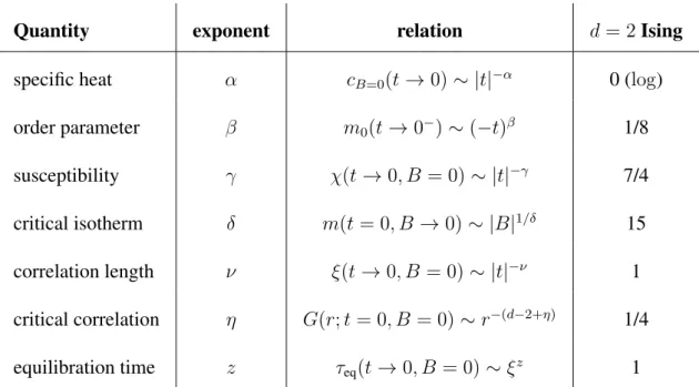
One of the most significant applications of classical thermodynamics is in the study of phase transitions. In this case, divergences and other singularities appear in the second (or higher order) derivative of the free energy.
Thermal phase transitions
This non-conservation of a symmetry of the Hamiltonian in the statistical mean hσiibel below the critical point is denoted as spontaneous symmetry breaking. We are now in a position to discuss the issue with the magnitude of the free energy (1.3) near the critical point.
Quantum phase transitions
Therefore, TC on the classical partition function represents a measure of the quantum fluctuations in the equivalent quantum system. For example, at zero temperature and near the quantum critical point, the ground state energy per particle satisfies [51,52].
![Figure 1.1: Behavior of the two lowest energy levels of H(g) as a function of g. In (a) [H 0 , H 1 ] = 0, and there is a level crossing](https://thumb-eu.123doks.com/thumbv2/123dok_br/19547557.0/29.892.133.736.156.340/figure-behavior-lowest-energy-levels-function-level-crossing.webp)
Hamiltonian diagonalization and gap
From (2.32) we get that the ground state energy in the positive parity subspace is given by. We are now in a position to analyze the ground state energy gap in this model.
Work and entropy production in unitary drives
Consequently, at the end of the drive, the final non-equilibrium state of the system will be given by (von Neumann) the entropy change in the system is given by ρτ⊗ρthE) ln ρthτ ⊗ρthE and so.

Stochastic approach and fluctuation theorems
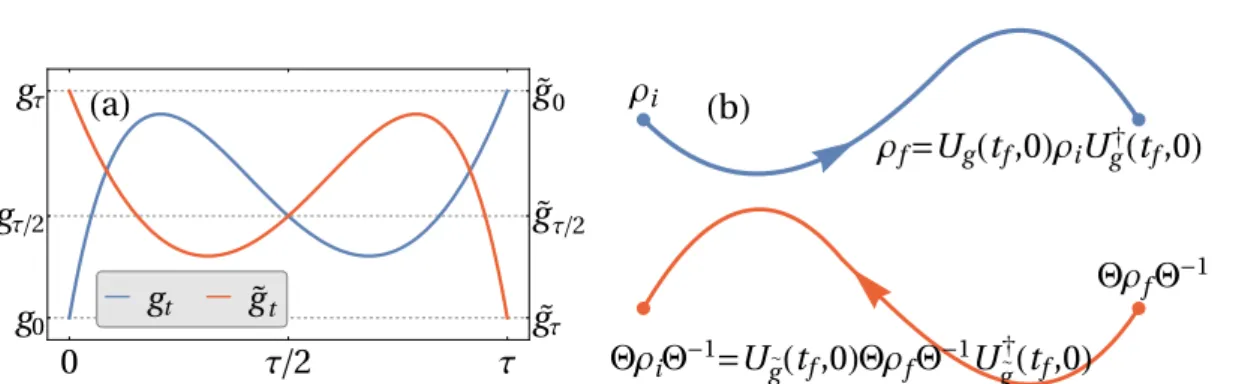
As a result of the feedback measurement, the system state is updated to. The work done on the system in a particular realization of the protocol is thus defined as. 3.26). Let us assume that the Hamiltonian of the system H(g) is invariant with respect to the reversal of time: ΘHΘ−1 = H; or in the case that H depends on the magnetic field B, that ΘH(B)Θ−1 = H(−B).
In the time-reversed protocol, the time sequence of the work parameter values is reversed: g˜t = gτ−t. After measurement, the state of the system is updated toρ˜τj = (1/rjτ)Πτj and then evolves according to unitary U˜g until time t = τ. The Hamiltonian of the system at the end of the time-reversal process, when the second energy measurement is performed, is H(g0).
That is, the fluctuations of the stochastic work w generated by the move include information about the equilibrium quantities. This method also enables to avoid performing two design energy measurements at the beginning and at the end of the work protocol.
Entropy production in the quantum Ising model
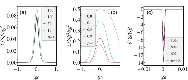
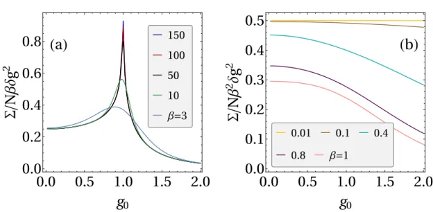
In Fig.3.3 it is shown the behavior of the entropy production as a function of the initial field g0 at several inverse temperatures β. As a consequence, there is an increase in the production of entropy near the critical point. To conclude our analysis of the behavior of the entropy production in the vicinity of a second-order quantum critical point, we note that the above result is obviously more general.
In this way, the behavior of the entropy production in the vicinity of the blue dot will not be spoiled by the adjacent second-order critical points. In Fig.3.5(c) the behavior of the second derivative of the entropy production with respect to the initial field g0 is shown. In this case, there is a discontinuity in the work as a function of the control parameter at the transition point in the limit T →0.
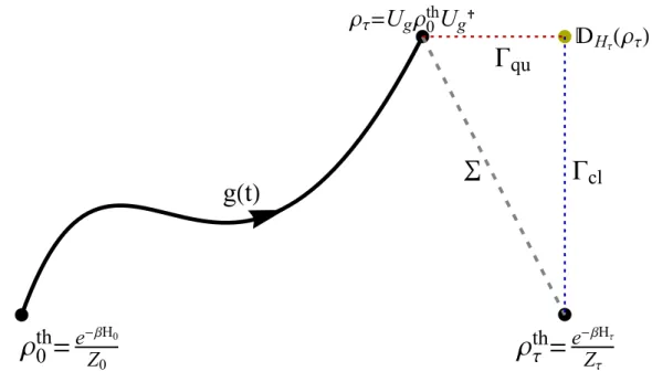
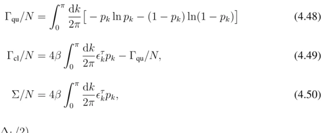
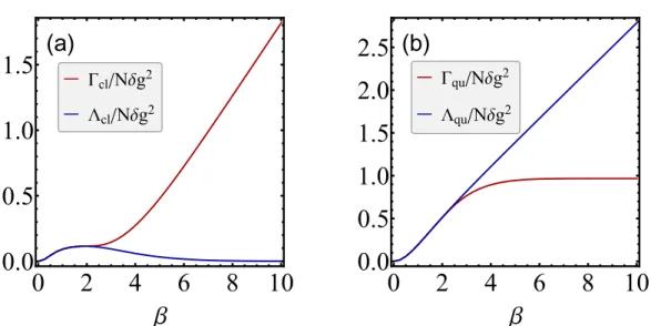
Then Γqu quantifies the contribution to entropy production arising from the energy coherences contained in the system state, ρτ, at the end of the drive. Now the final state of the system at the end of the work protocol, out of phase in the finite energy basis, can be written as
Γ-splitting in the quantum Ising model
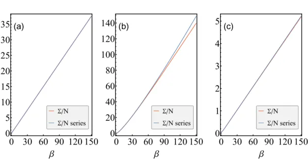
At the beginning of the work protocol, the system is prepared in a thermal state. We are now ready to calculate the two components of the entropy production (4.2) and (4.3) in a quenched Ising model. This finiteness of the coherence contribution to the spin entropy production is illustrated by the β → ∞ curve in Fig.
Furthermore, the creation of excitations near a quantum critical point at low temperatures is captured by the population part of the entropy production in the Γ splitting. 3.3, the entropy production becomes a flat function of the initial field at high temperatures and small quench sizes. For now, let us return to the analysis of the behavior at high temperatures.
This is expected following the previous discussion about the low-temperature behavior of this distribution of the entropy production. Nevertheless, there is still a significant increase of Γqu/Σ in the vicinity of the critical field value g0 = 1.
Shortcomings of the Γ-splitting
The contribution Γqu is supposed to measure how much of the entropy produces steam from quantum drag. These shortcomings of the Γ partition can be complementary analyzed from the perspective of its stochastic version [37]. At the stochastic level, the problem of analyticity of the Γ partition comes from the expression — see Eq.
The essential ingredient in the definition of the Γ-splitting was the introduction of an intermediate state DHτ(ρτ). This is nothing but the state of the system at the end of the run, ρτ, dephased with respect to the final Hamiltonian, Hτ. 5.3) Here, the eigenprojectorsΠ˜τi of the stateττ are connected to the eigenprojectors of the initial thermal stateρth0 (and the HamiltonianH0) through.
This is a thermal state based solely on the incoherent part of the finite Hamiltonian Hτ on the eigenbasis afρτ. This completes the formulation of our new partitioning of the entropy production following a working protocol.
Instantaneous and infinitesimal quenches
So, in summary, the shortcomings of the Γ-distribution discussed in Sect.4.2 disappear in the Λ-distribution. As another consequence, the creation of coherences further implies a break in the Gaussianity of the entropy production probability distribution [12]. As previously mentioned and shown at the end of the section, the variance, or second cumulant, of the entropy production is given by h(σ−Σ)2i=β2Var0[∆H].
To increase order on β, we can substitute the projector thermal state ρth0 on the ground state of the initial Hamiltonian, Π0i. After discussing the properties of the Λ-splitting in the instantaneous and infinitesimal quenching protocol at the level of means, let us next consider its stochastic formulation. Therefore, the limit|sj|<1 needed for the analysis of the Γ quantities quickly saturates with decreasing temperatures.
The CGF partition of the entropy production in (5.54) was first noticed in [12], where the authors were studying a quasi-isothermal process as a series of quantum quenches. An interesting feature of the Γ- and Λ-splits of entropy production is the fact that they coincide at temperatures high enough for instantaneous and infinitesimal quenching.
Λ-splitting in the quantum Ising model
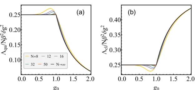
Moving on, let us consider the distribution Λ in the vicinity of the critical Ising point at (g = 1, h= 0). In the splitting Λ, this is the contribution related to the subsequent divergence of the total entropy production in the limit T → 0 (β. In contrast, pk can be considered equivalently as a measure of the rotation in its own energy basis resulting from extinction [ 37].
It is evident in the above equation the presence of the derivative of the ground state energy ∂g000 multiplied by a continuous function of β and 0i. This concludes the analysis on the behavior of ΛclandΛquin in the vicinity of the critical Ising point at (g = 1, h= 0). This is similar to its behavior near the Ising critical point discussed earlier.
Therefore, these first derivatives of the kink singularity in the middle of the Hamiltonian spectrum are imprinted on Λcl and Λqu at high temperatures. This completes the analysis of the Λ-splitting of the entropy production near both types of critical points in the alternating transverse field Ising model.
Experimental evaluation of Λ cl and Λ qu
This shows the Λ quantities give a true glimpse of the spectrum of the system Hamiltonian at high temperatures. The former indicates the change in equilibrium free energy associated with incoherent part of the perturbation∆Hd =P. It is clear that f is also a function of the initial field g0, but I omit this to simplify the notation. 5,102).
Of course, as I showed in Chapter 3, in the case of higher-order quantum critical points, it is a derivative of the entropy production that diverges in this limit. In particular, the dominance of the 'classical' part at low temperatures and highly coherent protocols and the failure of analyticity when no such problem arises in the total entropy production. In this scenario, the classical and quantum parts of the new splitting are inextricably linked.
For a system with a linear dependence on the control parameter, this is respectively equivalent to a relation to the first derivatives of the unperturbed eigenvalues of the energy and the eigenbasis. Reversals to the classical and quantum parts of the split occur even in protocols performed at arbitrarily high temperatures and mean that they can function as valid detectors of quantum critical points.
Gap Expressions
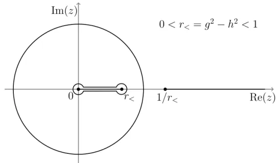
In this appendix, I give the steps necessary to obtain the gap expressions from Section 2.1. To solve this integral, we cut the branch in the interval (0, r<)∪(1/r<,∞) and deform the integration contour. For other intervals for which 0 6= |g2 −h2| 6= 1, basically we follow the same steps, adjusting the cuts of the branches.
Bounds on the gap
In this Appendix I review some of the concepts of quantum mechanics and quantum information theory applicable to this thesis. The von Neumman entropy can therefore be interpreted as the measure of state mixing. Therefore, relative entropy is considered as a measure of the difference between two quantum states.
The difference is that the initial incoherent state of the environment must be a thermal state. However, at low temperatures and in the ferromagnetic region, g < 1, Zc+ corresponds to only half of the total partition function ZF. The curves are quiet close to each other with a small difference in the vicinity of the critical field g0 = 1.
Effects of the Dzyaloshinsky-Moriya interaction on non-equilibrium thermodynamics of the XY chain in a transverse field. Pointer basis for the quantum apparatus, into which mixture does the wave packet collapse? Physical examination D.