In addition, a form for the heat fluctuation theorems was also studied in the case where there is also a flux of particles, and its validity. In the context of open quantum systems, dephasing is responsible for the loss of cohesion.
Linear Algebra for Quantum Mechanics
- Linear Operators and Matrices
- Inner and Outer Products
- Completeness Relation
- Eigenvalues and Eigenvectors
- Commutator and Anticommutator
- Adjoint and Hermitian Operators
- Trace
The basis of {|vii} vector space is such that every vector in this space can be written as an angle. LINEAR ALGEBRA FOR QUANTUM MECHANICS In terms of components in the basis, it becomes an inner product.
Postulates of Quantum Mechanics
Mean Value of an Observable
The mean value of the observed A, given that the state is |ψi, is written ashAiψ or simply hAi. Given that the operator A has a discrete spectrum with eigenvalues an, the mean value is hAi=X.
Solution of Schrödinger’s Equation
A very important basis is that formed by the eigenstates of the Hamiltonian, obtained by solving.
Time Evolution Operator
Density Matrix
Properties of Density Matrix
Another useful quantity is the trace of ρ2, which is defined as the purity of the system. For a pure ensemble this is trivial because ρ2 =ρ so the trace will clearly be the same, but for a mixed ensemble the purity will be less than one and hence the trace of ρ2 serves as a measure of the purity of a state.
Von-Neumann Equation
When a quadratic form is always non-negative for a state |φi, this immediately implies that the operator itself must be positive.
Tensor Products and Reduced Density Matrix
Tensor Products
Given the spaces HA and HB and their bases, let us take an operator O(A) belonging to HA and O0(B) belonging to HB. A convenient and clearer way to represent an operator O(A) ⊗ O0(B) is the matrix representation, known as the Kroenecker product.
Partial Trace and Reduced Density Matrix
TENSOR PRODUCTS AND REDUCED DENSITY MATRICES We thus see from this result that, from the perspective of system A, we can write the expectation value of an operator as an expectation value over a mixed state, described by the density matrix. Let us now return to the original proposition, with a condition ρAB =|ψihψ|, where|ψi is given by Eq.(2.81).
Interaction Picture
Entropy and Mutual Information
2.108) is the starting point for quantifying the degree of correlation between two systems by means of mutual information. Mutual information as a function of individual entropies and total entropy and is defined by [36].
Introduction to Second Quantization
INTRODUCTION TO THE SECOND QUANTIZATION imagine a system with N particles of the Hamiltonian H, whose eigenstates |nν1, nν2, nν3, ..i, where nνi are bounded by Pinνi =N, completely describe the state of the system, where νi are the states in which a particle can and i N is the number of states it can occupy. We do not have any problems for one-particle states, but for multi-particle systems it is necessary to take into account the symmetrization and antisymmetrization of the states.
Tight binding model
Two Site Problem
To understand the idea behind these techniques, let's first imagine a simple problem. If we are dealing with bosons, it is not a problem to have more than one particle per site, but with fermions the Pauli exclusion principle must be observed. The solution to the eigenvalue equation in this case is not immediately clear, but the idea is to find a transformation that makes the Hamiltonian diagonal.
One dimentional chain
Diagonalizing the Hamiltonian
It is possible to write any quadratic (in the creation and destruction operators) Hamiltonian as follows: 3.41) e.g. corresponds to the tri-diagonal matrix. There are two forms to treat a 1D chain. The first is called open boundary conditions and is an open chain, as shown in Figure 3-1. The other shape is called periodic boundary conditions, which is a circle formed by the intersection of the first and the last location.
Earlier we did an ansatz to get the sum of b†kbk to solve this problem.
Solving for a full chain
In the case of two sites we could do a simple ansatz that diagonalized the Hamiltonian. Even though the particle number operator does not appear directly in the Hamiltonian, it is interesting to see that our transformation does not change the number of particles. Now we look at the exchange conditions contained in the Hamiltoniana†i+1ai and a†iai+1 a†iai+1 = 1.
A DIMENSIONAL CHAIN For the expression Pia†iai+1 it is enough to take the dagger from the equation above.
Grand Canonical Ensemble
- Formulation of the Grand Canonical Ensemble
- Occupation Number and Internal Energy for Fermions
- Thermodynamics Limit
- Sommerfeld Expansion
- Sommerfeld Expansion in the Internal Energy
- Affinities and fluxes
- Markovian Systems
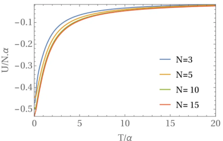
Opening the large partition function in terms of the occupation of each state and the total number of particles, we find. By examining the changes in the internal energy, it is possible to know properties such as heat capacity or heat flows or even particle flows. We can see through Eq.(3.105) that when|µ| →2, the value of the internal energy diverges in the Sommerfeld expansion. The smaller the value of |µ| is, the better the approximation will be.
The other central quantity in this framework is the response of the system to the affinities, which are characterized by the flows of the extensive quantities Xk:.

Fluctuations theorems
Jarzynski’s Classical and Quantum Fluctuation Theorems for Heat
2In this section I use the sub-indexes f and b with the meaning forward and backward as a reference for the development of the process. To prove the quantum version, we continue with the first part of the protocol. As a result of the measurement, the systems A and B are projected onto a pure state |nA,Bi.
Once the systems are initially uncorrelated, the initial state of the overall system is given by|nAnBi.
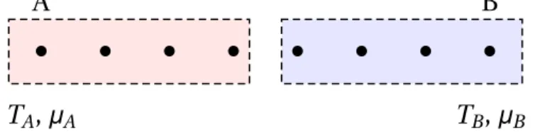
Fluctuation Theorems for Heat and Particle Exchanges for Bipartite
If the interaction energy is small compared to the energy of the systems, we say that we have a weak coupling. Mathematically, we obtain the time-evolved matrix of the system ρs through the application of a dynamic map, such that 1 [58]. If the evolution obeys the semigroup property, the evolution map is given by .
To derive another form of the main equation, we move the problem to Liouville space.
Mean values at non-unitary dynamics
The first term on the right is responsible for the unitary evolution and the same is obtained in the von-Neumann equation. It is also possible to obtain the time evolution of the average of the operators in non-unitary dynamics. Let's begin to more clearly identify the first term on the right side of the equation.
So the unitary part of the evolution of the system is just the average of the commutator of the Hamiltonian with the operator, which is nothing but Heisenberg's equation for closed systems.
Decoherence and Dephasing Noise
The link with the environment now defines cohesion, a measure of the quantumness of the system. DECOHERENCE AND DEPHASING NOISE Therefore, the time evolution of the density matrix is given by. Thus, the dephasing sound can be interpreted as a relaxation with no exchange of energy, once the populations are constant, in the basis of the Hamiltonian.
These facts will be important in the construction of the phenomenological dephasing used in this thesis.
Fluxes and Onsager Coefficients
- Thermodynamic Limit and Final Fluxes
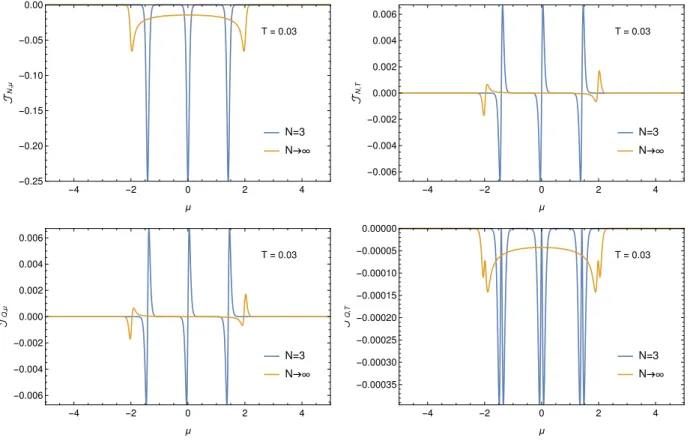
- Final Fluxes for Finite Chains
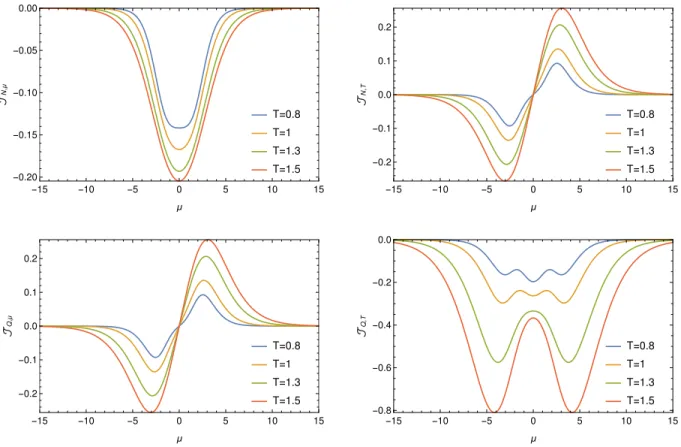
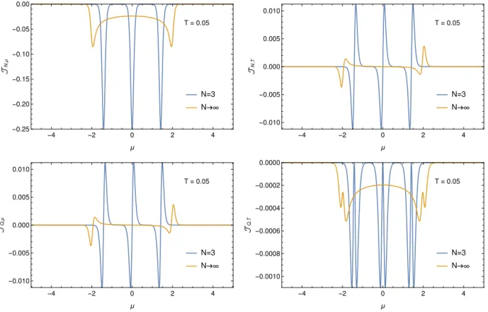
- Analysis for Fixed µ
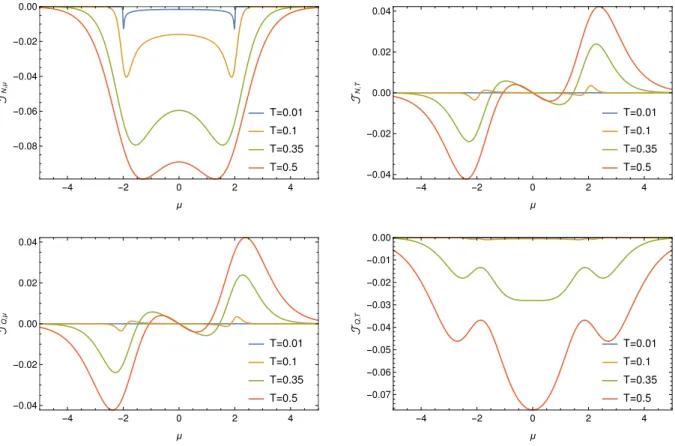
- Analysis for Fixed T
- Time-Dependent Fluxes
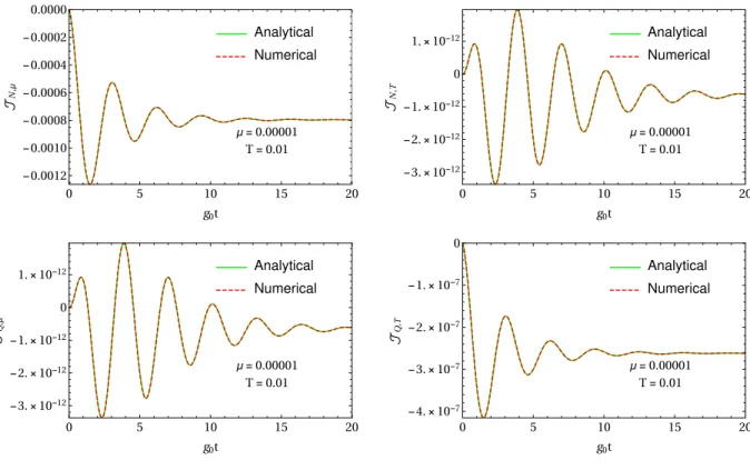
- Analytical Solution for Low Temperatures
The parity of the currents can be explained by the parity of the energy band. Now we can go further and analyze the dependence of flows on the number of cities. We can now use Figure (6.8) to analyze the effect of temperature on these peaks/valleys.
Finally, we also address the typical evolution of the system in the case without fading.
Entropies and Mutual Information
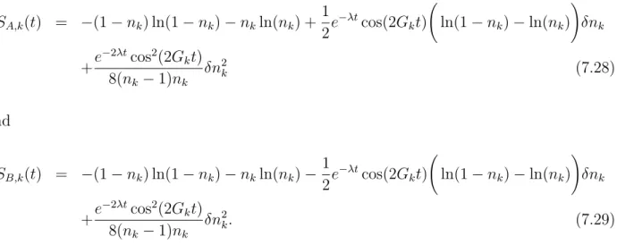
Entropies for the individual chains
The term independent of δnk is exactly the value of the entropy of equilibrium, which is intuitive because the equilibrium will occur with occupation nk and the first order inδnk term means the amount of entropy exchanged. In Fig. (7.1) it is already possible to notice the role of damping of the dephasing. For systems with the dephasing some entropy is produced and this is more evident for the case with dephasing shown in 7.2.
Moreover, as can be seen in Figure (7.3), the different states do not interfere with the equilibrium state, but only with evolution.
Entropy of the Total System for a Momentum k
ENTROPIES AND MUTUAL INFORMATION of the system. ha†kakithb†kbkit)2+ha†kbkithb†kakit(nA,k−nB,k)2. ha†kakithb†kbkit)2+ha†kbkithb†kakit(nA,k−nB,k)2. 7.30). Since the occupations will be in equilibrium for a long time, so will the entropy. One important thing is that production is not only positive, but not just zero for systems affected by a dephasing, as evidenced by the.
ENTROPY AND MUTUAL INFORMATION dependence of Π on λ and in figure (7.4). a) Total entropy of the system.
Mutual Information
EXCHANGE PROBABILITY FOR A MOMENTUM Then it is possible to see that the mutual information shows that the systems begin.
Exchange Probability for a Momentum k
As expected, the particle-free state and the completely occupied state do not evolve because the number of particles is conserved and the Pauli exclusion principle is obeyed. The one-particle states are initially uncorrelated, but once the systems A and B interact, these states will become correlated. This correlation disappears by the action of the dephasing, which for a long time will make both states equally likely.

Fluctuation Theorem for the Bipartite System
Fluctuation Theorem for the Momentum k
So this result agrees with the fluctuation theorem for the exchange of energy and matter, with the exchange of energy and particles expected with the assumptions.
Fluctuation theorem for the Full System
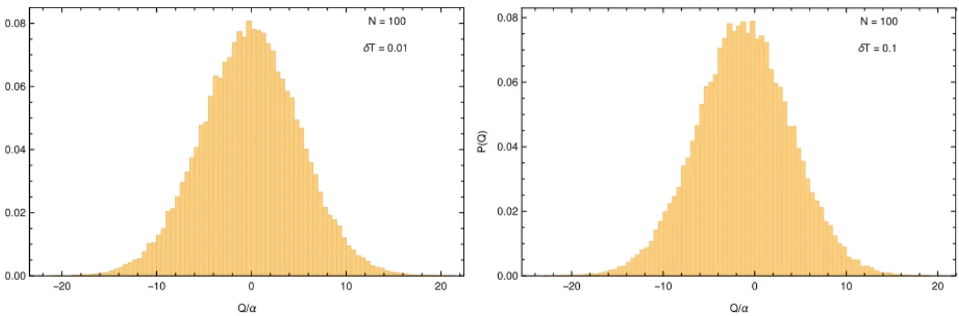
Probability Distribution of Heat
PROBABILITY DISTRIBUTION OF HEAT with the same temperature and number of places, but differentδT, we see a deviation of the curve. As said before, with the decoupling of the energy levels, it was possible to check that the whole system also obeys an exchange-fluctuation theorem. The distribution of heat can then tell us the importance of the original occupation in the statistics of the system.
In this appendix I discuss a particular function that was used to find an analytical solution for the evolution of the system when we start with low temperatures.
Recurrence Relations
Bessel’s Differential Equation
Integral Picture
In this section, I show only a few images that were used to study the validity of the analytical solutions. 2In the last step for I1 and I2 I used the exponential form of the cosines to make obtaining the results easier. Bustamante, "Verification of the rogue fluctuation theorem and recovery of rna folding free energies," Nature, vol.
Klümper, „Thermodinamics of that Anisotropy Spin-1/2 Heisenberg Chain and Related Quantum Chains“, Journal for Physics B Condensed Matter, vol.