A thesis submitted in conformity with the requirements for the degree of Masters in

I would like to express my deepest appreciation to all those who have directly or indirectly supported and helped me during the realization of this thesis. First, I would like to express my sincere thanks to my supervisor, Doctor Andr ´e Marta, for his constant encouragement, support, invaluable advice, guidance and interest in discussions throughout the course of this work. On a personal level, I would like to thank my friends for their support and understanding regarding my absence in the last months.

Finally, I would like to express my deep gratitude to my family, especially my parents, for all their support and presence during my academic and military course. Palavras-chave: quantificaç ão de incercito, Monte Carlo, hipercubo de Latin, m étodo das perturbaç ões, elementos finitos, projecto robusto.

Nomenclature

Glossary

Introduction

Motivation
Importance of Uncertainty Quantification
Relevance to Aeronautic
Aircraft Structures

Wing Structures
Wing Materials

Thesis Outline

In the process of uncertainty quantification, the last stage is the validation of the model, so there are also many studies on this subject [Alvin et al., 1999]. In recent years, UQ has gained strong importance in the aviation industry and studies. Including uncertainty in CDF simulations has gained importance in recent years.

More recently, there are other materials used in the aerospace field, such as titanium alloys and fiber-reinforced composites. After this, some statistical concepts that will be used in the UQ methods are presented.

Uncertainty Quantification

Ranks and Process of Uncertainty Quantification

It can also be called reducible because additional information about the system can reduce its influence on the final response. Model uncertainty is also a result of a lack of information, but in this case it is a result of not understanding the behavior of the variables or some simplifications introduced into the model. Identification is essential to determine sources of uncertainty, either from the system or its environment.

Without it, both the quantification of uncertainty and the system analysis will be compromised. With the variable correctly identified and characterized, it is possible to propagate the uncertainty through the system and understand how it responds.

Statistical Concepts

Mean, Variance, Standard Deviation and Covariance
Probability Distribution

It is the average value of the squared deviations with respect to the simple mean [Murteira et al., 2007], defined as. This measure is important because it shows how far the set of numbers or distribution is from the mean value and is an important parameter for describing a probability distribution (see section 2.2.2). It is another important tool to characterize the probability distribution as its value indicates how far the distribution is from the mean value.

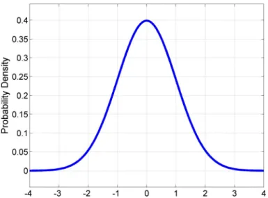
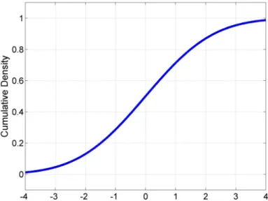
From the PDF graph it is possible to know the probability associated with a particular value of the answer. From the CDF graph it is possible to know the probability that the response value is in the range]− ∞;x].

Optimization with Uncertainty

Robust Design Optimization (RDO)
Reliability Based-Design Optimization (RBDO)

The goal of RDO is to optimize the response of the system in terms of the average values [Allen and Maute, 2005]. It maximizes the performance of the system by minimizing the sensitivities to the random variables. This minimization is translated by the reduction of the standard deviation of the system response along the mean.

The mean value (µf) and the variance (σ2f) of the quantities can be calculated if the variables are continuous or There is another approach to RBDO where the objective function is defined in terms of the probability, P, that the original function exceeds or does not exceed the required target [Allen and Maute, 2005].

Uncertainty Quantification Methods

Monte Carlo Simulation Method
Quasi-Monte Carlo Simulation Method
Latin Hypercube Sampling Method
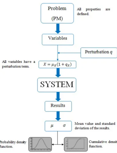
Perturbation Method
Fast Probability Integrator

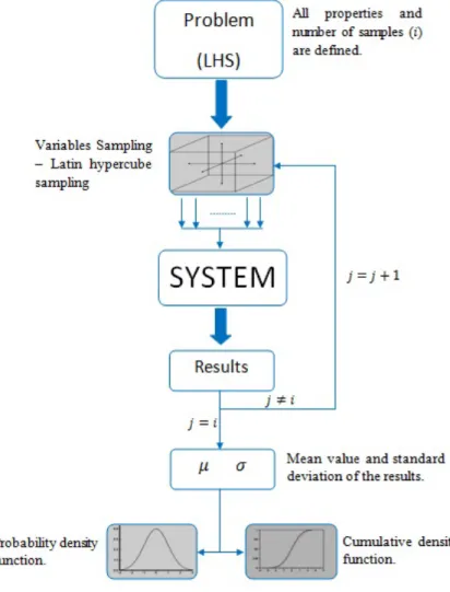
Since MCS is a method whose base is statistics, it is necessary to solve the problem many times to achieve the desired accuracy. First, it is necessary to properly define the problem, its variables, and the number of samples needed to achieve the desired accuracy. It begins with the sample of each variable and it is necessary to know their mean and standard deviation.

Once the output results have been processed, it is possible to plot the CDF and PDF for each output. With a stratified sample it is possible to achieve accurate results with fewer samples, which reduces the computational effort. Usually, first and second order derivatives with respect to the primitive random variables are used, but it is necessary to ensure that the covariance of the random variables is small [Wei, 2006].

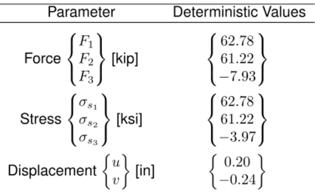
In the second order, it is necessary that the coefficient of variance is less than 20% [Sudret and Kiureghian, 2000]. For the input variables, it is necessary to know their mean and covariance, not the standard de-. 3.7), it is possible to notice that the average value for the first-order approximation corresponds to the average value obtained from a deterministic analysis.

Given the covariance matrix, it is easy to obtain the standard deviation of the system since it is equal to the square root of the main diagonal of the covariance matrix. Comparing the equations for the first (Equ. 3.11)), it is possible to see that the average value for the second order has an additional term. For complex systems, it is very difficult or even impossible to obtain the system equations analytically; instead, finite difference approximations may have to be used.

Three-Bar Truss

Model Description
Deterministic Analytical Analysis
Monte Carlo Simulation Method
Latin Hypercube Sampling Method
Perturbation Method
Discussion of Results

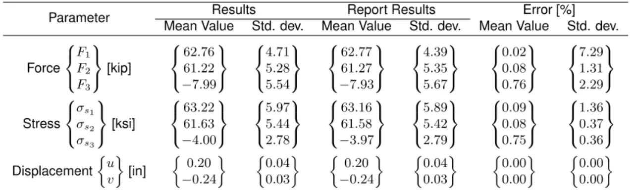
Once the case has been fully described, it is possible to start applying the UQ methods. After the simulation, it is possible to get the results for different number of samples. Comparing the results, it can be observed that the mean value represents a good match, but the standard deviation shows a not so good match.

However, the purpose of this comparison is to compare the results obtained from the implemented method and the reference report. By analyzing results, it is possible to observe that the calculated results and report results agree very well. Comparing the simulation time, LHS is significantly faster than MCS and the results are very close.

When all primitive variables are defined, it is possible to do the Taylor expansion, as illustrated. Observing the results, it is possible to see that the results produced offer a very good agreement with the results in the reference report. The biggest difference observed in the results is in standard deviation and it is about 6%, the smallest being less than 0.02%.

After the implementation of the selected methods, a comparison of the results between them is required, Tab. 4.5 shows a comparison between the results obtained for each method. By comparing the results, it can be concluded that three different methods present very close results. Making a general comparison using the results of the graphs shown in Fig. 4.4, it can be observed that the obtained results show a very good agreement.

Wing Spar

Model Description
Deterministic Analytical Analysis
Sampling Convergence Study
Stochastic Analytical Analysis
Deterministic Numerical Analysis
Stochastic Numerical Analysis

After integration, it is necessary to determine the constants using the boundary conditions of the problem. With the expressions for maximum displacement and maximum stress, it is possible to apply the developed UQ methods to obtain the mean value and standard deviation of these responses. After the convergence study, it is possible to run the simulation and obtain the results with the required accuracy.

To validate the use of FEM, it is necessary to compare the results obtained from analytical and numerical analyses. After model validation, it is possible to study the wing spat with the UQ methods developed in Chap. By comparing the expressions for the first derivative (Eq. 5.17), it is possible to observe that they are different.

From this comparison, it is possible to see that the difference is a constant term, corresponding to the mean value of the variable that was differentiated. By using these methods, it is possible to obtain the mean and standard deviation of the required outputs. As referred to in the analytical analysis, the computation time of PM is less than that observed in the other methods.

5.4, it is possible to observe that the results for each method are very close, moreover, they generally offer good accuracy. Observing the maximum displacement PDF distributions, it is possible to see that all the distributions present a low possibility of the displacement taking positive values. With these results it is intended to show the influence of the uncertainty in the input parameters.

Wing Structure

Model Description
FEM Convergence Study
Deterministic Numerical Analysis
Stochastic Numerical Analysis
Comparison of Computational Cost

With these properties it was possible to obtain the aerodynamic response of the wing. Therefore, it is necessary to perform an interpolation between the results of XFLR5® to obtain the results for the node location in the ANSYS® mesh. The figure illustrates the structure, load distribution and wing constraints at the root.

Before starting the analyzes with UQ methods, it is essential to do a convergence study in terms of the number of elements. Finally, it is possible to do the deterministic analysis and obtain the results for the desired accuracy. Maximum stress (tension) is observed on the underside and the minimum (compression) is in the upper plane of the wing.

Analyzing the deterministic results, it can be concluded that the structure did not suffer damage under this load because the maximum stress observed on the wing is less than the ultimate tensile strength and the tensile yield strength. Since this structure is more complex than the wing flap, a convergence study is required for the number of samples in the MCS and LHS sampling methods. If we compare the accuracy of the results for the wing structure analysis and the wing flap analysis, in this case the results are closer than the results for the wing spar analysis.

By comparing the PDF for each method, it is possible to verify that the results from the different methods are very close. With them it is also possible to see that the results are very close to each output. Since the wing structure has a certain complexity, it is practical to make an analysis of the computational cost.

Conclusions

Achievements

By comparing the deterministic and the stochastic results, it was possible to show that the uncertainty in the input affects the output, as their average values increase motivated by the uncertainty. The implemented methods could be used to design wing structures with input uncertainty, and if a workstation with strong computational capabilities is used, it will be possible to use these methods to design structures more complex, closer to reality. Overall, the knowledge acquired within UQ with this thesis can be used in future construction projects, leading to better, more robust and reliable solutions.

Future Work

Bibliography

An overview of recent developments in the numerical solution of stochastic partial differential equations (stochastic finite elements). On the Use of Quasi-Monte Carlo Methods in Computational Finance, Book Title = Computational Science - ICCS 2001. A comparison of three methods for selecting values of input variables in the analysis of the output of a computer code.

Appendix A

ANSYS Script for the Wing Model Analysis

Appendix B

MATLAB Script for the Monte Carlo Simulation Method

Appendix C

MATLAB Script for the Latin Hypercube Sampling Method

Appendix D

MATLAB Script for the Perturbation Method