Die gemeinsame Wahrscheinlichkeitsverteilung ist für den Analysten sehr nützlich und kann nur in seltenen Fällen analytisch ermittelt werden. Es ist erwiesen, dass die Berücksichtigung von Abhängigkeiten (z. B. in Ereignissen oder in Modellen) einen erheblichen Einfluss auf das Ergebnis hat.
Problem definition
One of the main projects within this period is the GHI (2004) RADIUS (Risk Assessment Tools for Diagnosing Urban Areas Against Seismic Disasters) project. The proposed methodology allows a consistent representation of the effect of dependencies on loss estimation for important buildings (eg hospitals).
Objectives
Scope and outline of the dissertation
The aggregation of losses can be performed assuming a purely linear consequence model (i.e. for residential buildings, the damage to one building does not influence the consequences of the damage to another building) or any kind of non-linear consequence model (i.e. the collapse of a hospital). has a significant impact on the overall impact of another hospital's damage, as the lack of treatment capacity can lead to additional indirect losses for the society in question). Examples of the application of the functional system concept can be found in cybernetics (Mesarovic and Takahara, 1975), of the structural system concept in Klir (1972) and of the hierarchical system concept in combination with structural system concepts in Lin (1999).
Decision theory
The alternative with the maximum is the optimal decision. αis a measure of the pessimism of the decision maker. Von Neumann and Morgenstern (1944) state a set of axioms, the fulfillment of which enables the allocation of numerical values (utility) to the preferences of the decision maker.
Uncertainty, probability, utility and risk
None of the existing loss estimation methodologies explicitly consider the dominant parameters by considering their uncertainty. None of the aforementioned seismic loss estimation methodologies take into account such a comprehensive approach to knowledge.

Proposed framework
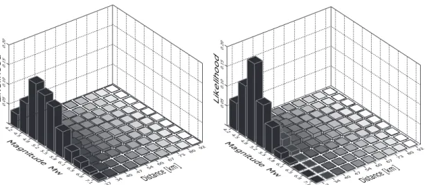
In Figure 4.3 the BPN for seismic hazard analysis of a generic line source is illustrated with the marginal distribution of spectral displacement. The correlation of ground motion intensity parameters PGA and SD(T), which is used in the development of BPN models, was developed based on Baker (2007).

Soil failure
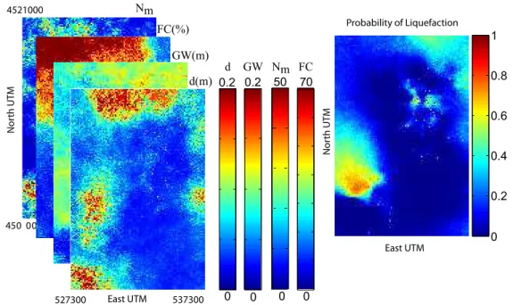
Thus, the necessary parameters for the evaluation of liquefaction initiation are the SPT impact number Nm, the fines contentFC, the soil classification according to the Unified Soil Classification SystemU SCS, the water table GW and the depth of the critical layer. For those locations where all the necessary parameters are available, the probability of liquefaction can be calculated. Kriging aims to reduce the standard deviation of the difference between the estimated and the true value.
The variogram, denoted by γ(h) is equal to the variance of the increase in data points separated by a distance h. For each distance and direction, pairs are derived from the samples and half of the variance of the differences in the data pairs is calculated. In the region of Adapazari, Turkey, the soil properties are required for each of the grid points of 100 x 150 elements with a dimension of 100 m x 100 m.
For each of the combinations (M,PGA) the probability of liquefaction is calculated for each grid point. The output files of the simulations are read into MATLAB with the files Depth_field.m,USCS_.

Structural damage
It is assumed that the structural performance of the buildings is adequately represented by generic reinforced concrete frames (Figure 4.21). The open source finite element program OpenSees is used to calculate the structural response (OpenSees, 2008). The dynamic properties of the replacement SDOF systems are assigned according to the relationships proposed by Priestley (1998) and the TDY (1998).
It will be assumed that the residual displacements calculated for a replacement SDOF system can be used as an estimate for the remaining displacements of the buildings in the corresponding structural class. These two structural response parameters together can provide a good idea of the seismic performance of a structure. The calculation scheme of the seismic vulnerability curve for the structure classes is shown in Figure 4.25.
Estimation of the parameters of the lognormal distribution for the set of SDs in each damage condition using maximum likelihood. Classification of the 320 MIDRs and the corresponding SDs of the time history given the damage performance limits.

Consequences
The method was first developed by Ciriacy-Wantrup (1947) and used for estimating the statistical value of life, e.g. The Revealed Preference Method estimates the best solution based on consumer behavior. An overview of the applications of this theory for estimating the statistical value of life is given in Blaeij et al.
The LQI is consistent with consumption theory and provides a consistent method for estimating the statistical value of life. The fatality ratio is the number of people killed in relation to the number of occupants in a building. Coburn and Spence (2002) provide five M-factors to estimate the number of deaths that can occur in an earthquake (Figure 4.26).
In evaluating the examples, data on the number of floors and floor area are used to estimate the number of victims of each building. The data on the number of residents for each building is then included in the GIS platform for each building in the city and evaluated using the BPN for the consequence model (Figure 4.27).

Verification and validation of the models
The BPN seismic hazard model in Figure 4.5 is applied with the characteristics of the Kocaeli earthquake of 17 August 1999. The main result of BPN structural damage is in the form of discrete probabilities for three damage states (no damage, repairable damage, collapse). Therefore, the calculated earthquake risks must be multiplied by the occurrence rate of earthquakes greater than Mw=5.0 for each of the seismic sources.
The BPN evaluation was performed in a GIS environment using the commercial software Hugin (2008). Figure 5.7 shows the optimal response for each building using the time-dependent seismic hazard. The optimal retrofit decision for each building in the city is calculated using the scheme given in Figure 5.8.
The minimum of the total expected cost indicated the optimal decision for each structure (Figure 5.6). The minimum of the total expected cost indicated the optimal decision for each structure (Figure 5.7).

Example 2: Assessment of seismic risk
The total expected cost for the portfolio is calculated by adding the expected cost of the buildings. In other words, these nodes are independent of the corresponding nodes in the other buildings. For the three general nodes considered (i.e. size, distance and fragility curve uncertainty) the composition of the loss exceedance curve is illustrated in Figure 5.12.
The size probability distribution is hardly different for the first years, here for 2009. For comparison, the existence of shared nodes is ignored, and the node 'Cost' distribution for each building is evaluated for stand-alone BPNs using the CostDistS2_ file. The 'CostS2' node distribution is calculated by sampling the 'Cost' node distributions for each of the 1246 buildings using the file Aggregation_Poisson_S2_Integrated.m.
The discrete probabilities of the node 'Cost S2' representing the portfolio loss due to seismic source S2 are simulated using a. The distribution of the node 'Cost' for each building is evaluated For each combination of.

Example 3: Update of fragility curves
Starting with the first of the 201 buildings, the BPN is further conditioned on the use of information on the liquefaction condition and structural damage condition of the first building. The two nodes 'Liquefaction' and 'Damage' are properly instantiated and the parameters of the fragility curves are updated using BPN. The probability distributions of the uncertainty nodes are updated using the Hugin software in a GIS environment.
O_Res_RA_2.mber calculates the discrete probabilities for the states of the node 'Damage', given the states of the nodes 'Lambda Yellow', 'Zeta Yellow', 'Lambda Red' and 'Zeta Yellow', and the states of the node 'SD ' specified inBPN_PSHA_Adapazari_BU.m. For each of the 42 combinations of magnitude (6 states) and PGA (7 states), the probability of liquefaction at each grid point is calculated using the scheme in section 4.2. These probabilities were imported into GIS as 42 additional columns in the attribute table of the corresponding building class shape file.
This 201x2 matrix is read from the attribute table of the corresponding shapefile in GIS. Using the labels of the first building, the BPN is conditioned and the 'Lambda Yellow', 'Zeta Yellow', 'Lambda Red' and 'Zeta Yellow' nodes of the fragility curve are updated.

Example 4: Index of robustness
Defining the system as the entire region where the city of Adapazari is embedded results in a different composition of direct and indirect losses and thus a different resilience index. Sakarya region, the estimate of the macroeconomic costs of the Kocaeli Mw7.4 earthquake on August 17, 1999 is assumed to apply. 2000) estimates are given for the entire affected region of the Kocaeli Mw7.4 earthquake. To some extent, all the existing loss estimation methods can be considered as integrated approaches. The application of the proposed framework is illustrated using four examples of earthquake risk problems for.
The fourth example illustrates the use of the robustness index as an indicator. Methods and rules for a consistent representation of the effect of dependencies when estimating losses are developed. The unconditional and conditional probability tables (hereinafter referred to as potentials) for the variables in the considered BPN are shown in figure A.1.
For example, when the state of the "Liquefaction" node in the BPN in Figure A.1 is no longer uncertain, i.e. The domain graph in Figure A.7 is not a triangular graph; as mentioned above, eliminating the G variable requires a new connection. The input message is multiplied by the potential in the clique of the variable being considered.
The conditional probability table of the node 'SD' is initialized with. for all combinations of the states in the 'Magnitude' and 'Distance' node. the spectral shifts are calculated with the Boore Joyner and Fumal.