Can monetary policy be helped by domestic oil price stabilization?

No. 502

Can monetary policy be helped by

domestic oil price stabilization?

DEPARTAMENTO DE ECONOMIA

PUC-RIO

TEXTO PARA DISCUSSÃO

N

o

. 502

CAN MONETARY POLICY BE HELPED BY

DOMESTIC OIL PRICE STABILIZATION?

EDUARDO LOYO

LUCIANO VEREDA

Can monetary policy be helped by

domestic oil price stabilization?

Eduardo Loyo

∗

Luciano Vereda

#

November 2004

1. Introduction

In early 1999, international prices of crude oil stood at a long time low, after a two-year declining trend that brought them down by nearly 60%. Over the two following years, prices increased threefold, only to fall again by more than 40% in the space of one further year. One more year is all they took to recover fully the latter loss, but then they tumbled again by one-fourth in a couple of months. Since mid-2003, they have almost doubled, reaching by August 2004 a peak that was just shy of five times higher than the trough of early 1999.

Such a rollercoaster ride, especially the more recent escalation, did not pass unnoticed in economic policymaking circles. There has been some speculation about the US tapping their strategic oil reserves, for instance, with the objective of regulating supply to the domestic economy and containing the adverse impact of recent oil price hikes. There have also been scattered instances in which taxes levied on oil were adjusted in order to cushion international price movements, and an unknown number of instances in which similar ideas must have crossed the minds of policymakers but were ultimately not acted upon.1

Similar effects may also be delivered by the voluntary or enforced pricing policy of national oil monopolies, wherever they exist. Passing on to the domestic market less than the full movement in international prices may be consistent with profit-maximizing motives in face of a downward-sloping demand curve, even if there are no barriers to price adjustment. Meanwhile, nominal rigidities equally consistent with profit maximization discourage transmission of cost shocks expected to be short-lived. The oil monopoly can

∗

Banco Central do Brasil and Department of Economics, PUC-Rio ([email protected]). The views expressed here are not necessarily those of the board of directors of the Central Bank of Brazil. The authors are grateful to Pierpaolo Benigno, Afonso Bevilaqua, Tiago Cavalcanti, Márcio Garcia, Marc Giannoni, Affonso Celso Pastore and Michael Woodford for comments either on recent or on much earlier versions of this work. [This version 24/11/2004. Preliminary and incomplete. Omitted derivations and proofs can be obtained from the authors upon request. Please do not quote.]

#

Department of Economics, PUC-Rio ([email protected]).

1

also exercise an extra degree of smoothing in answer to non-commercial policy objectives of the shareholding or regulating government.

Here what we see is a new lease on life being given to an old policy debate: should national governments find ways to shield their domestic economies from oil price fluctuations taking place in the world market? Presumably, such insulation from the most egregious source of aggregate supply shocks could relieve some of the burden that would otherwise be shouldered by conventional tools of macroeconomic stabilization – notably monetary policy. Critics argue, in turn, that allowing domestic consumers to face price signals that reflect without distortion the terms on which scarce resources trade internationally would produce a more efficient allocation, at least in price-taking countries.

The aim of this paper is to put those contending positions to a more formal test. We do so in what has become the standard framework for the welfare analysis of macroeconomic policy stabilization (see Woodford, 2003). The analysis is performed in a parsimonious dynamic general equilibrium model of an economy with nominal rigidities. The conditions for equilibrium with rational expectations are explicitly derived from the maximizing behavior of households and firms. Those equations are written in terms of ‘deep’ parameters describing preferences and technology, which are thus taken to be invariant to the choice of policy regime. As a result, the model is ‘structural’ and arguably immune to the Lucas critique, as a policy evaluation exercise requires. Moreover, alternative policies are ranked not according to some ad hoc objective function, as was so common in the earlier literature on macroeconomic stabilization, but according to the welfare of the representative household who is assumed to inhabit the economy. The welfare criterion is derived from the household’s utility function, just as the dynamic behavior of the economy emerges from maximization of that same utility.

Policy evaluation performed in a framework in which the equilibrium behavior of the economy and the welfare criterion share a common set of microfoundations has long been standard practice in fields such as international trade and public finance. Although it is only natural that the same internally consistent approach should have been extended to the evaluation of macroeconomic stabilization policies, the extension is even more natural when it comes to the issues to be analyzed in this paper. After all – at the intuitive level of the policy debate at least – the contest pits the plausible objective of improving the output-inflation trade-off available to aggregate demand management against efficiency considerations regarding instruments of trade or taxation policy, fields in which that very approach is the established standard.

The focus on price misalignment caused by nominal rigidities raises an interesting possibility that goes against the grain of the whole debate about intervention in domestic oil prices: that it might actually be a good thing to exacerbate the oil price signals transmitted to the domestic economy, with respect to their fluctuations in international markets. Sticky prices of final goods and services having oil as an intermediate input would still adjust by less than the change in their marginal costs, as perceived by the price setters. But privately perceived marginal costs, thanks to exacerbating intervention, would change by more than the true social marginal cost – which is a function of the undistorted, international oil prices. The net result might be an adjustment of prices of final goods that is closer to what would be observed if these prices were fully flexible, and therefore less inefficiency from misalignment. The possible gains from exacerbating intervention will be explored in the analysis below, together with the more conventional aspects of the policy debate.

The paper is organized as follows. Section 2 reviews the standard new Keynesian model used in the monetary policy evaluation literature. Section 3 describes how that standard model is augmented for the analysis of the issues at hand. The most distinct feature of our baseline model is the existence of two internationally traded intermediate inputs, each used by a certain fraction of the producers of final goods. Section 4 reports the main results for that baseline economy. Section 5 takes a short detour through a model with an alternative specification of price rigidity, yielding different implications of inflation and of commodity price intervention for price misalignment and welfare. Although our baseline model contains the more conventional specification of price rigidity, the alternative specification sheds some valuable extra light on our results. Up to that point, our results are all analytical and robust to the calibration of the model.

Further progress can be made, though, with resort to numerical results from calibrated models. The numerical approach is particularly useful when we incorporate to our baseline model additional features that may enhance the beneficial role of commodity price intervention. We consider welfare criteria that directly penalize movements in the monetary policy instrument, and allow for shocks that change the degree of inefficiency of the economy, in the form of time variation in distortionary tax wedges. Section 6 explains the criteria by which we propose to judge whether intervention in the domestic prices of intermediate inputs can be a quantitatively important adjunct to monetary policy in those circumstances. We propose to compare the gains from adding this extra instrument to gains from making certain improvements in the recipe followed by the monetary authority in setting interest rates, which has been the focus of the monetary policy evaluation literature. Sections 7 and 8 contain the results of our quantitative investigation for calibrated economies. Section 9 concludes.

2. Modeling preliminaries

The most recent literature on the evaluation of macroeconomic stabilization policies – in particular, of monetary policies – relies on a simple dynamic general equilibrium model of aggregate supply and aggregate demand. The standard version is derived from the utility maximizing behavior of a representative, infinitely-lived household, and from the profit maximizing behavior of a large number of monopolistically competitive firms producing each a differentiated good.

The representative household cares about variety in its consumption basket, according to constant elasticity of substitution (CES) preferences across all differentiated goods. As a result, there is a well defined demand curve for each good, which is downward sloping in the relative price of that good. At the same time, the household suffers the disutility of supplying labor for production. Utility is supposed to be additively separable over time with a constant one-period discount factor.

Firms use labor as their sole input and are subject to restrictions on their ability to adjust prices. Nominal rigidities are typically modeled as in Calvo (1983): each period, a constant proportion of firms is randomly drawn to set new prices; each newly adjusted price becomes valid starting that same period and remains in force until the individual firm gets drawn again for another price adjustment. As a result, given the format of the demand curves for each good, firms will set new prices by applying a desired mark-up to a weighted average of current and future expected marginal costs. Once a price is posted, firms are assumed to satisfy all forthcoming demand.

The probability of an individual firm being drawn to set a new price is independent of how misaligned the firm’s going price is or of the time elapsed since the firm was last given the chance to adjust. This setup, though clearly artificial, allows for a parsimonious stylization of an economy with time-dependent, staggered price setting, without the need for a large state space describing the pricing history of each firm. The model is typically parametrized to allow for an adequate degree of strategic complementarity among pricing decisions (firms that do adjust prices do so by less than they would if all other firms were also adjusting in the same direction), which enhances the real effects of nominal shocks and enables the model to match the observed behavior of real-world economies.

These elements lead to a dynamic system with rational expectations. The much greater ease of computing rational expectations solutions to linear than to nonlinear models implies that the model is most often represented by a first-order approximation to the true equilibrium conditions. In that linearized format, the model contains the dynamic versions of an aggregate supply and an aggregate demand curve:

t t t t

t =κx +βEπ +1+u

π [1]

(

t t t t

)

t t

t E x R E r

Equation [1], describing aggregate supply, is the standard new Keynesian version of the Phillips curve. It relates inflation π_t (the change in prices between t-1 and t) to the output

gapx_t. The presence of a term involving inflation expectations is a familiar feature of expectations-augmented Phillips curves, but note that here we have the current expectation of future inflation, not the past expectation of current inflation. This is so because new prices entering into effect at time t also depend on what firms expect the general price level to be in the future, when their current price will remain in force with some probability.2 All future inflations matter, as the Phillips curve creates a chained link by which π_t+1 depends

on E_tπ_t+2, π_t+2 on E_t+2π_t+3, and so forth indefinitely.

The output gap is just the difference between actual output and potential output, while the latter is precisely defined as the level of output that would obtain in equilibrium if all prices in the economy were flexible. Potential output is an exogenous variable that may change through time according to, say, changes in productivity or shifts in the labor supply curve. Such regular supply shocks, however, do not perturb the relation between inflation and the output gap captured by the Phillips curve.

To understand why, it is important to know that the output gap stands in the Phillips curve as a proxy for real marginal costs, which naturally affect inflation because pricing decisions result from applying a desired mark-up over marginal costs. Real marginal costs increase with the level of output because an increasing marginal disutility of labor implies that real wages are pushed up in order to elicit greater labor supply; depending on how the production technology is specified, it may also increase because firms face upward sloping marginal cost curves (given the prices of inputs). On the other hand, a shock that shifts marginal cost curves downwards (implying lower marginal costs for any given level of production) increases the flex-price equilibrium level of output, our definition of potential output. Up to a linear approximation, the increase in marginal costs associated with higher actual output and the decrease associated with higher potential output are exactly symmetric, turning the output gap into a proper proxy for marginal costs.

Ordinary supply shocks that simply change marginal costs do affect inflation – a channel that is captured by the presence of the output gap in the Phillips curve – but they do not affect the relation between marginal costs – or their proxy the output gap – and inflation. However, one can readily conceive of supply shocks that would indeed perturb the relation between marginal costs and inflation. Anything that changes the wedge between prices and marginal costs would have that property. Examples would be changes in tax rates levied on production inputs or output, or changes in the firms’ desired mark-up. Because changes in distortionary taxation or in the market power of producers are inherently changes in the degree of inefficiency of the economy – in particular, changes in the degree of inefficiency of the potential level of output – those have been termed by Woodford ‘inefficient shocks’

2

in connection with the new Keynesian Phillips curve. Inefficient shocks are collected under the rightmost term u_t, which appears, as expected, as an exogenous perturbation to the relation between inflation and the output gap.

The aggregate demand equation [2] is derived from the Euler equation for the dynamic optimality of consumption plans, relating intertemporal allocation between the present and the future to the ex-ante real interest rate R_t −E_tπ_t+1 accruing in the meantime (R_t is the one-period nominal interest rate between t and t+1, contracted on nominal bonds at time t). Because it is a relation between the dynamics of level of activity and the interest rate, it is sometimes called the ‘intertemporal IS curve’. Here the Euler equation is already written in terms of the output gap instead of the level of output or consumption. This is convenient because the level of activity then appears in the demand curve measured by the same variable as in the Phillips curve [1].

The substitution of the output gap for the level of consumption in the Euler equation increases the number of exogenous terms in the equation, to include potential output alongside demand shocks such as government expenditures in goods and services. That composite exogenous shock is collected under the term r_t, which then lends itself to a nice interpretation: it is the ex-ante real interest rate consistent with a constant output gap, that is, with output moving in tandem with potential output, just as it would do if all prices were flexible. Woodford (2003) associates this term with the Wicksellian concept of ‘natural rate of interest’.

The same microfoundations lead to a welfare loss criterion of the form:

∑

∞ =0 +

s

s t s

t L

E β [3]

where 0<β <1 is the representative household’s intertemporal discount factor and:

2 2

t t

t x

L = +ψπ [4]

is the period loss function. That is obtained as a quadratic approximation to the exact loss function resulting from the microfoundations. Policy evaluation is based on ranking equilibria that satisfy the linearized relations [1]-[2] according to the quadratic criterion [3]-[4].

Of course, in the absence of distortionary taxation, that condition will not be satisfied in an economy where firms enjoy market power. The maintained assumption is that some sort of distortionary taxation is employed to undo the effects of market power. Usually, a subsidy to marginal costs is assumed to be present at a precisely calibrated rate, so that firms applying their desired mark-up to the subsidized marginal costs would end up practicing prices equal to the true (unsubsidized) social marginal cost of production. As a result, shocks to distortionary taxation present among the inefficient shocks u_t should be interpreted as departures from the subsidy rates that make potential output coincide with the perfectly competitive output level.

It is noteworthy that the quadratic approximation to the welfare criterion represented by [4] should be so close to the ad hoc objective functions typically assigned to monetary authorities, penalizing a weighted sum of quadratic deviations of inflation and the level of activity. However, along a number of dimensions [4] contains much more structure than its

ad hoc predecessors. First, it is the fluctuation of the output gap, measured with respect with a precisely defined concept of potential output, which is penalized. That may be very different from penalizing fluctuations in the actual level of output or in the departure of actual output from some trend, for potential output is recognized to be time-varying and the desirable behavior then becomes to make actual output move in tandem with potential, so that x_t can be as small as possible in absolute value.

Second, the whole linear-quadratic approximation leading to equations [1] to [4] is performed around a steady state with zero inflation, which means that the term π_t appearing in the approximations is none other than the rate of inflation itself. As a result, [4] indicates that departures from zero inflation are penalized, not departures from some other arbitrarily chosen inflation target. That zero should be the optimal rate of inflation is understandable in this economy since the welfare loss stemming from inflation is entirely due to the price misalignment caused by nominal rigidities, as transactions frictions (a transactions motive to hold non-interest bearing monetary balances) are assumed either to be absent or to make a negligible contribution to the welfare criterion.3 Price misalignment is obviously minimized when inflation never causes prices to need adjustment, that is, when it is zero.

3

Third, the relative weight ψ in the period loss function is not an additional degree of freedom in the parametrization of the model, but is instead fully determined by the model’s preference and technology parameters. As a matter of fact, it has been found that a compelling calibration of those parameters yields a value for ψ that is large compared to relative weights often assigned to inflation in ad hoc versions of loss functions of the same form as [4] (see Woodford, 2003).

An important property of this standard model economy is that complete stabilization of both inflation and the output gap is possible if there are no inefficient supply shocks: if

0

≡

t

u , equations [1] and [2] are consistent with x_t ≡π_t ≡0, provided only that monetary policy makes the nominal interest rate follow the path of the natural rate of interest (R_t ≡r_t). Complete stabilization of these two variables is obviously optimal in terms of welfare, as can be seen immediately in equation [4]. It does not mean, of course, that output is being stabilized, as it is actually being made to replicate the exogenous trajectory of potential output, so that the output gap remains always equal to zero. Demand shocks or supply shocks that do not affect the degree of inefficiency of potential output are not an impediment to such complete stabilization.

The truly essential lesson, however, is that the welfare criterion must be consistent with the same microfoundations from which the equations describing the equilibrium dynamics of the economy are derived. Naïve application of the same loss function [4] to an economy with a different structure may produce seriously misleading results in terms of policy evaluation. The next section describes how the baseline model [1]-[4] can be adapted to the analysis of price intervention policies. The new features incorporated into the augmented model will be reflected both in its behavioral equations and in the matching welfare criterion.

3. Intermediate inputs and international trade

The standard new Keynesian model just described does not lend itself to the investigation of the effects of intervening in domestic commodity prices in face of international price fluctuations. Here we follow the strategy of making the minimal necessary modification to the standard model in order to be able to address the issues at hand.

To keep our initial motivation in mind, we shall refer to one of these commodities as ‘oil’, and to the other as ‘grain’. Final consumer goods are produced with a very simple technology, with constant returns to scale and fixed proportions of labor and one intermediate input, either grain or oil. Grain is used as an input by a fraction η of the final goods producers (0<η<1), and oil is used by the remaining 1−η. Labor is homogeneous in the entire economy.

Increases in the domestic price of oil relatively to the domestic price of grain induce final goods producers, applying a mark-up over their marginal costs, to charge relatively higher prices for the goods that have oil as an input. The prices of the final goods determine the quantities in which they are demanded, which ultimately determine the domestic absorption of oil and grain.

We shall denote by ε_t the logarithmic difference between the international prices of grain and oil – in other words, it is a linear approximation to the relative price of grain in terms of oil in international markets. In the absence of any barrier to trade, the domestic relative price of the two commodities would also be ε_t, but we want to allow for intervention causing the log difference between the prices of grain and oil in the domestic market to be

t

t λ

ε + instead, where λ_t is a linear approximation to the wedge created by policy between domestic and international relative prices.

Both commodities could in principle be produced domestically using only homogeneous labor as an input, each through a simple technology with constant returns. The economy is assumed to be small, a price-taker in world commodity markets. We also assume that the relative productivity between the domestic production of the two commodities and the probability distribution of international relative prices are such that the economy completely specializes every period in the production of grain, even when the relative price of grain in international markets is at its lowest. The economy will thus export grain in order to be able to import oil. Since oil is necessary for the production of a certain range of final goods, and since CES preferences (same as in the standard model) do not allow for equilibrium with zero supply of any final good, equilibria will always involve oil imports.

For the sake of simplicity, we require the economy to maintain a zero trade balance every period. The possibility of intertemporal trade, with the economy cyclically accumulating or drawing down assets against the rest of the world, would open some extra degrees of freedom for the intertemporal allocation of domestic absorption, but it would remain true that, in present discounted value, the economy would be able to spend as much on oil imports as it earns in grain exports. The absence of intertemporal trade assumed here avoids the discussion of more complicated issues of current account sustainability while at the same time it imposes a meaningful budget constraint on the economy’s dealings with the rest of the world.

Now it is convenient to define potential output as the level of output that would obtain if all prices were flexible and if there were no barriers to trade (λ_t ≡0). Among the exogenous

international commodity markets. When ε_t is high, potential output is also high, for the grain producing economy faces more favorable terms of trade in that case and, as a result, the overall quantity of intermediate inputs it can afford increases.

Just as in the standard model, potential output will only be efficient if some sort of distortionary taxation is used to undo the effects of market power by producers of final goods. We assume that the appropriate subsidy to the marginal costs of production is in place to induce monopolistic competitors to produce the same quantities as competitive firms would if faced with the same real wages and intermediate input prices, at least in the steady state around which we take the linear-quadratic approximation to the exact equations of the model. We allow for stationary departures from that optimal level of taxation, which are then regarded as inefficient shocks appearing in the aggregate supply relation.

With the above modifications, we obtain aggregate demand and aggregate supply equations that have the exact same format as [1] and [2], with the proviso that the output gap is now calculated with respect the level of output that would prevail with flexible prices and free trade. Now, however, we identify a specific source of inefficient supply shock, namely the departures from free trade measured by λ_t. For instance, if there is no time variation in desired mark-ups, but we allow the rate of taxation on the marginal costs of production (away from the optimal tax rate, which we know is negative) to vary, the inefficient supply shock in equation [1] will be:

(

)

t

t t

u =ωτ − 1−η γδλ [5]

where ω, γ and δ are all strictly positive structural parameters and τ_t is the departure from the optimal tax rate on marginal costs. It is assumed throughout that the tax rate on marginal costs is non-discriminatory, that is, it applies equally to all producers of final goods. In particular, the parameter γ measures the degree of price flexibility in the economy,4 while δ is a parameter related to labor productivity.5

First, it is important to note the absence of any term in ε_t in equation [5]. Variations in the relative prices of commodities in international markets are supply shocks, and as such, as already mentioned, they are reflected in potential output. They do not, however, constitute an inefficient shock: neither do they change the relation between profit-maximizing prices and marginal costs in the final goods sectors, nor do they affect the ability of our precise definition of the output gap to proxy for marginal costs in the economy as a whole. So, variation in the domestic relative prices of commodities, insofar as it reflects variation in

4

It is a increasing function of the proportion of firms, in Calvo’s formulation, randomly drawn each period to adjust prices. Apart from that proportion, it depends only on the one-period discount factor β.

5

the terms of trade, do not put any pressure on inflation, either up or down, beyond that already represented by changes in the output gap. Nor does such variation create an impediment to the complete stabilization of inflation and of the output gap, although it would clearly cause potential output to fluctuate and thus require actual output to fluctuate in the same proportion for the output gap to remain stable.

On the other hand, [5] also reveals that variations in λ_t do constitute inefficient shocks. In particular, intervention increasing the domestic relative price of grain (decreasing the domestic relative price of oil) is a negative inefficient shock, that is, it puts downward pressure on current inflation given the output gap and expected future inflation. That conclusion holds regardless of the relative importance of grain and oil as intermediate inputs in the economy, measured by 0<η<1, although the impact will be stronger the more important the oil processing sector is (the smaller is η), and will tend to vanish as the economy approaches the limit in which all final goods producers process grain only.

The reason for the asymmetric roles of oil and grain prices is that the domestic price of grain is linked to the wage rate (recall that labor is homogeneous) through the marginal equality between revenues and costs of the perfectly competitive domestic producers of grain. There is no similar connection for oil prices, since oil is not produced domestically. If domestic oil prices were to vary in the same proportion as domestic grain prices and wage rates, that would have an impact on inflation through marginal costs, but not on the relation between inflation and marginal costs, as proxied by the output gap. On the other hand, changes in domestic oil prices relative to grain prices and wage rates could in principle represent a perturbation to the relation between inflation and the output gap, the importance of which would naturally be greater the larger is the participation of the oil processing sector in the economy. However, if such relative price changes mirror the variation in the terms of trade, they are also reflected in fluctuations of potential output, and so it is through the output gap that their impact on inflation will show. In the end, only relative changes in domestic oil prices due to intervention appear as a perturbation to the Phillips curve, that is, as an inefficient supply shock. In particular, intervention reducing domestic oil prices relatively to domestic grain prices and wage rates causes a decrease in the average marginal costs throughout the economy that is not proxied by the output gap, and hence its appearance as an extra term in the Phillips curve pushing inflation downwards.

At this point we can also note from equation [5] that commodity price intervention and non-discriminatory taxation can be jointly varied in such a way as not to generate an inefficient supply shock. In particular, if non-discriminatory tax rates vary for some reason, commodity price intervention could in principle be used to undo – or at least to mitigate – the inefficient shock, a topic to which we shall return in section 8 below. Likewise, if commodity price intervention is taking place, changes in non-discriminatory taxation could in principle be used to undo the inefficient supply shock, and we shall refer to this property in the next section.

(

)(

[

)

2

(

)

2

]

1

2 2

1 _{t t t t}

t t

t x p p p

L = +ψπ +ψη −η − ₋ +γ −δε [6]

where p_t is a linear approximation to the average relative price of consumer goods that use grain as an input with respect to the average price of consumer goods that use oil as an input, and ψ is again a positive weight fully determined by the structural parameters of the

model. The extra terms appearing in [6] besides those already present in [4] represent the welfare loss from price misalignment that is not measured by the overall inflation rate. Note that, if the economy approached the limiting cases in which all producers of final goods process the same intermediate input (η →0 or η→1), the loss function would also approach that of the standard one-sector model.

The two terms inside the square brackets in [6] have each an intuitive interpretation. It can be verified that, if all consumer prices were flexible, the equilibrium relative price of goods produced with grain would be:

(

t t

)

t

p =δ ε +λ [7]

If trade was also free (λ_t ≡0), the rightmost term in [6] would be identically zero under flexible prices. That term can thus be interpreted as a measure of misalignment between the average price of grain processors and oil processors, to which we shall refer as intersectoral

price misalignment.

But nominal rigidities also causes price misalignment within each sector, as some firms processing grain do adjust prices to prevailing marginal cost conditions while others are prevented from following suit, and likewise among firms processing oil. We refer to that as

intrasectoral misalignment – or intrasectoral dispersion, since alignment among firms facing the same marginal costs requires that they all charge the same prices. If all firms in the economy always faced the same marginal costs, the degree of intrasectoral dispersion would be fully determined by the overall rate of inflation, as in equation [6], because all firms adjusting prices would always be moving towards the same desired price.

Because the path ofp_t has a direct impact on the welfare criterion, a policy evaluation exercise must also take into account how that path is affected by exogenous shocks, policy instruments and, perhaps, the equilibrium values of other endogenous variables like inflation and the output gap. It can be shown that the dynamics of p_t is governed by:

(

)

t t

(

t t

)

t

tp p p

E β γ γδ ε λ

β + + + − = +

− ₊₁ 1 ₋₁ [8]

The relative price of goods in the grain-processing sector responds to the domestic price of grain relative to oil, which is formed by the international relative price ε_t and the wedge λ_t

generated by commodity price intervention. The dynamics of p_t does not depend on anything else; in particular, given its own initial condition and the current and expected future path of ε_t +λ_t, it is independent of other endogenous variables in the economy. As a

result, the only way policy can interfere with the trajectory of p_t is through commodity price intervention.6

Equation [8] can be solved separately from the rest of the model for the rational expectations equilibrium response of p_t to an innovation in the stochastic process ε_t +λ_t.

If ε_t +λ_t remains permanently constant at any given value, p_t eventually converges to the

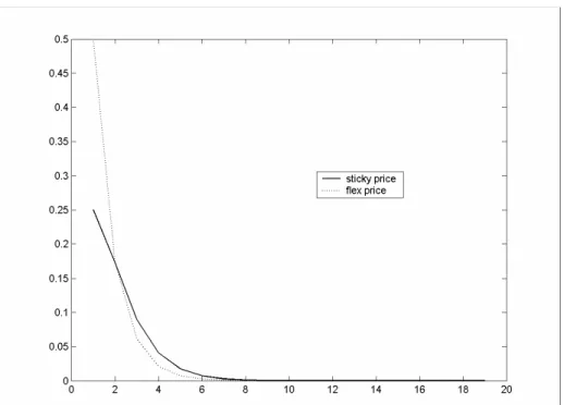
flex-price level described by equation [7]. If ε_t +λ_t follows a mean-reverting stochastic process with some persistence – say, to make it more precise, an AR(1) process – then an innovation to that process immediately impacts p_t in the same direction, but less so than it

would if prices were flexible. Reversion of p_t to steady state is faster under flexible prices

(case in which it would have the same persistence as ε_t +λ_t), and after some point in time

the flex-price path of p_t would actually be closer to steady state than its sticky-price path. Just as an illustration, Figures 1.1 and 1.2 display the flex-price and sticky-price responses of p_t to an innovation in ε_t +λ_t, respectively characterized by [7] and by the solution to

[8], under the assumption that ε_t +λ_t follows an AR(1) process (with autoregressive coefficient 0.35 or 0.70).

4. Results in a baseline economy

Suppose that we have an economy described by equations [1], [2], [5] and [8], in which the welfare loss is measured by [3] and [6]. In this section we study the optimal macroeconomic stabilization plan in this economy, with or without the collaboration of intervention in domestic relative prices of commodities.

6

The rational expectations solution to this expectational difference equation starting at any given time t = 0 must satisfy an arbitrary initial condition for p-1. The characteristic polynomial of the equation has exactly one

stable and one unstable root, implying that the equation has a unique bounded solution satisfying that arbitrary initial condition. The solution for pt , for every non-negative date t, is then a function of pt-1 and of the time t

Consider first what the best possible macroeconomic stabilization plan would be if there were no departures from optimal non-discriminatory taxation (τ_t ≡0), and if there was no

commodity price intervention either (λ_t ≡0). In the absence of intervention, the trajectory

of p_t determined by equation [8] would be entirely independent of policy, a function of the

exogenous trajectory of ε_t alone. As a result, the two terms inside the square brackets in equation [6] would themselves be independent of policy, and policy choice could equivalently be guided by minimization of [3] with the simpler period loss function [4].

With 0u_t ≡ (direct consequence of τ_t ≡λ_t ≡0, according to [5]), the solution to this problem is trivial, as seen in section 2: to stabilize inflation and the output gap completely, letting the nominal interest rate always be equal to the natural rate. Shocks to the international relative price of commodities ε_t do have an impact on welfare – which is properly measured by [6], not [4] – through both intrasectoral and intersectoral price misalignment arising from fluctuations in p_t, but there is nothing the conventional instruments of macroeconomic stabilization can do about it.

Consider then the main question we want to answer regarding this baseline model economy: whether manipulation of policy instrument λ_t can improve welfare compared to that obtainable under free trade. One can easily verify that, in the absence of departures from optimal non-discriminatory taxation (τ_t ≡0), the answer to that question is a clear ‘no’.

In order to prove that claim, the first step is to find the unrestricted choice of trajectory

{ }

pt _t≥0 that minimizes:

(

)

(

)

[

]

∑

∞ = − − + − 0 2 2 1 0 t t t t t t p p p

E β γ δε [9]

which can be recognized as the welfare loss function [3] with a partial period loss function given by the terms inside the square brackets in [6]. The first-order conditions to this simple dynamic minimization problem reduce to:

(

)

_{t t t}

t

tp p p

E β γ γδε

β + + + − =

− ₊₁ 1 [10]

which is none other than the equation characterizing the sticky-price dynamics of p_t under

free trade – that is, equation [8] with λ_t ≡0. Because the rational expectations solution of

[8] is uniquely determined and is a function of

{

ε_t +λ_t

}

_t≥0, free trade is both necessary and sufficient for the solution of [8] to satisfy the optimality condition [10]. Any departure from free trade would thus be inferior as far as the partial criterion [9] is concerned.

stabilization of inflation and output gap (x_t ≡π_t ≡0) consistent with the Phillips curve [1] and with the intertemporal IS curve requiring that the nominal interest rate replicate the trajectory of the natural rate of interest. Complete stabilization of inflation and output gap reduces to zero all terms in the period loss function [6] that were not already counted in criterion [9], while free trade already minimized the latter, so free trade is indeed the optimum according to welfare function as a whole. In conclusion, commodity price intervention cannot be of help under the circumstances considered so far.

In this economy, intervention produces two separate effects. First, it interferes with the trajectory of the relative price of final goods, as measured by p_t, which has a direct impact on welfare through price misalignment. Second, it generates an inefficient shock – namely, a change in the economywide average marginal costs of final goods that is not reflected in the output gap. As a result, one might have intuited that a possible case for free trade would have relied on the adverse impact of the inefficient shock – which renders complete stabilization of inflation and of the output gap incompatible with the Phillips curve – being perhaps so strong as to overwhelm the possibly beneficial effect, in terms of price misalignment, of departing from the free-trade path of p_t.

Quite to the contrary, the proof just presented of the optimality of free trade shows that the result is actually stronger, in that it does not depend at all on intervention having the adverse side-effect of an inefficient shock. Intervention would still be bad even if one could undo its inefficient shock effects by deft manipulation of τ_t, assuming that

(

)

_t

t ω ηδλ

τ ≡ − −

1

1

instead of τ_t ≡0. That would entail u_t ≡0, and absence of inefficient shocks allows for complete stabilization of inflation and output gap, regardless of what happens to international commodity prices or to intervention in their domestic prices (those variables would vanish from the Phillips curve). Both ε_t and λ_t would matter solely for the

determination of the trajectory of p_t, according to the expectational difference equation

[8]. The policy problem would then reduce to choosing, alongside x_t ≡π_t ≡0 (with

t

t r

R ≡ ), the trajectory of λ_t that minimizes [9]. That trajectory, we already know, is

0

≡

t λ .

As a matter of fact, the result is stronger still, since the free trade path of p_t characterized

by [10] is the unrestricted optimum, not simply the best trajectory of p_t that can be

generated by manipulation of λ_t according to the solution to equation [8]. Even if the

relative price p_t of final goods could be directly dictated by the social planner, instead of being merely induced by intervention in the relative price of their intermediate inputs, no trajectory of p_t would be preferable than the one spontaneously arising from free trade.7

7

Because the trajectory of ptdefined by [10] is the unrestricted minimizer of [9], one also concludes that, in

our sticky price economy, the intersectoral relative price pt had better be left to its naturally sticky behavior,

The partial welfare criterion [9] suggests that two contrary forces are at work here, which combined render free trade optimal in terms of minimizing the degree of price misalignment arising from each given rate of inflation. On the one hand, the first term inside the square brackets in [9] is smaller the more dampened the movements in p_t are, a

purpose that is served by reducing λ_t wheneverε_t increases, so that the domestic relative price of the commodities does not fluctuate so much. Smaller movements in domestic relative commodity prices mean less inducement for relative prices of final goods to change, and thus reduces the intrasectoral price dispersion that would arise if they did change (for, in each sector, some firms would be changing while others would be left behind). That would militate in favor of using intervention to cushion the domestic economy from the worldwide fluctuations of commodity prices.

On the other hand, the more dampened the fluctuations inp_t become, the farther away they would be from following their flex-price, free-trade behavior, which would then increase intersectoral price misalignment, captured by the second term inside the square brackets in [9]. For instance, it can be readily verified that, if ε_t follows a stationary AR(1) process

with autoregressive coefficient ρ, and the trajectory of p_t is governed by equation [8], then the intersectoral price misalignment term in [9] is completely eliminated by setting:

(

)

1

1 1

1

−

− −

+

= _{t t}

t γ ε γ ε

ρ β

λ [11]

This expression reveals that the policy that minimizes intersectoral misalignment, given the lagged value ε_t−1 on which it also depends, reacts to an increase in ε_t with a further

increase in λ_t.8 In other words, it exacerbates the fluctuations in domestic relative prices of commodities compared to what they would be if they simply reflected the international price fluctuations. The exacerbated movements of relative marginal costs would induce greater adjustment of the intersectoral relative price, to the point of replicating the flex-price trajectory [7] for the average relative price across sectors, in spite of the presence of nominal rigidities. That, however, would come at the cost of much greater intrasectoral dispersion of prices.

Figure 2 illustrates this trade-off numerically, assuming that λ_t =θε_t and computing the unconditional expectation of each of the two terms inside the square brackets of [9] for

the period loss function would no longer be given by [6]. In particular, the social planner should never dictate individual prices entailing any intrasectoral price dispersion, regardless of what she intended to do to the intersectoral relative price. Given that behavior, welfare would depend only on the output gap and on intersectoral price dispersion, and the latter would be minimized by the flex-price path of pt. The conclusion

that the sticky price behavior of pt is optimal holds only under the assumption that pt could be dictated by the

social planner, but that the behavior of the full set of prices of final goods by which such trajectory of pt

would materialize would still be such as to entail the welfare-reducing misalignment captured in [6].

8

different values of θ between –1 and 1. The first term (intrasectoral dispersion not captured by the overall inflation rate) is annulled when θ =−1, so that shocks to the terms of trade are perfectly offset (ε_t +λ_t ≡0) and p_t never budges; that component of intrasectoral dispersion increases monotonically with θ. Meanwhile, the second term inside the square brackets in [9] is minimized for some value θ >0, indicating that, within the class

t t θε

λ = , intervention that minimizes intersectoral misalignment is indeed of the exacerbating type. The two contending forces – intersectoral misalignment demanding exacerbation, intrasectoral dispersion demanding mitigation – exactly balance each other out in the sense that the sum of the two terms is minimized precisely when θ =0.9

The non-interventionist result obtained for our baseline economy – meaning that one wants neither to dampen nor to exacerbate fluctuations in domestic commodity prices – reflects that precise balance in the trade-off between intrasectoral and intersectoral price misalignment. This may strike the reader as quite a coincidence, suggesting that the result might not be robust to changes in certain assumptions of the model. In that regard, it must be noted first of all that the result does not depend on the numerical values of the model parameters, including the fraction of firms that process each commodity, and in this sense it

is generic.

Moreover, it is only under the assumption that non-discriminatory taxation offsets the inefficient shock caused by intervention that the perfect tie between intrasectoral and intersectoral misalignment considerations is particularly relevant in building the case for free trade. If intervention does produce an inefficient shock that is not offset, that acts as a further argument against departures from λ_t ≡0 in either direction, and might presumably render free trade optimal even if the trade-off between intrasectoral and intersectoral misalignment, taken in isolation, happened to recommend some marginal exacerbating or mitigating intervention.

There are, however, two dimensions along which changes in the structure of the economy might indeed change results. First, one might consider more than two commodities, and thus more than one relative price in which policy can intervene. With many commodities, each being processed by a sector that is very small relatively to the overall economy, intrasectoral price dispersion naturally becomes less important compared to intersectoral misalignment. In the limiting case of each differentiated final good resulting from processing a different commodity, there would be no intrasectoral dispersion, and all misalignment would be intersectoral by construction. Of course, intervening simultaneously in many relative prices severely complicates the problem both in theory and in practical implementation. If anything, however, it would imply greater encouragement for exacerbating intervention, since that helps mitigate the intersectoral misalignment that would have gained in relative importance.

9

Second, it is possible that different conclusions would arise from a different specification of price stickiness. Nominal rigidities of a different sort might well imply different implications of inflation and commodity price intervention for price misalignment, and thus lead to a different prescription for intervention policy. We have adopted the formulation of Calvo (1983), on which the vast majority of the monetary policy evaluation literature relies to derive not only the Phillips curve but also the implications of inflation for price dispersion and welfare. In the next section, we take a brief detour through a model derived from a different formulation of price stickiness, in order to gain further insight into the implications of commodity price intervention for welfare.

5. A detour: convex costs of price adjustment

Now we consider an economy in which nominal rigidities are modeled in the way proposed by Rotemberg (1982). All firms producing final goods are free to adjust prices every period, but they bear a cost that is a convex function of the size of the price adjustment. Convexity of the adjustment cost function implies that firms have an incentive to distribute any desired adjustment in a series of smaller steps rather than making a single larger movement.

In Rotemberg’s setup, firms are forward looking and choose at any date t =0 a trajectory of prices

{ }

P_{t t≥0} in order to minimize:

(

)

(

)

[

]

∑

∞ = − − + − 0 2 1 2 * 0 ~ t t t t t t P P P P

E β γ [12]

given an initial condition P₋₁ and the stochastic sequence of prices

{ }

* ₀

≥

t t

P that they would desire to charge at each date if there were no costs of price adjustment. The objective function [12] penalizes quadratic departures from the optimal price in the absence of nominal rigidities and the square of changes in prices from one date to the next. The parameter 0γ~> denotes the relative weight of these two penalties; since γ~−1 would be the relative weight of price changes, γ~ can be interpreted (just like γ in our baseline model) as the degree of price flexibility in this economy.

From that specification of price stickiness one can derive the following Phillips curve:

(

)

t

t t t

t κx βEπ η γδλ

π ~ ₁ ~

1− −

+

= ₊ [13]

under the assumption that the only source of inefficient supply shock is intervention in domestic relative commodity prices. Meanwhile, the dynamics of the intersectoral relative prices of final goods is governed by:

(

)

t t

(

t t

)

t

tp p p

E β γ γδ ε λ

β + + + − = +

− _{+ 1} ~ ₋ ~

1

Note that, apart from possible differences in the definition of certain coefficients, [13] and [14] have the exact same format as equations [1] and [8], respectively. Therefore, the dynamics arising from a Calvo (1983) economy could equally have been generated by an economy with Rotemberg-style sticky prices.

While the equations governing the dynamics of the economy share a common format, the welfare criterion is quite different between the Calvo and the Rotemberg models. Instead of [6], the Rotemberg formulation yields the following period loss function:

(

)

2

2 ~

t t t

t x p

L = +ψ −δε [15]

Note that, differently from [6], criterion [15] contains no terms in inflation or in the first difference of p_t. The absence is quite understandable since all firms facing the same marginal cost change prices in the same proportion period after period, and as a result there can be no intrasectoral price dispersion. The only source of price misalignment in the economy is the fact that relative changes in marginal costs across firms do not get immediately reflected in their relative prices. That is what we have been calling intersectoral price misalignment, which is measured by the rightmost term in [15] in pretty much the same way (apart from the different parametrization) as it appeared in [6].

Because overall inflation is of no direct consequence for welfare, the optimal plan in this case is to stabilize the output gap completely, letting inflation adjust in response to any inefficient shock appearing in the Phillips curve. If that is done, the only channel through which commodity price intervention λ_t can affect welfare is the dynamics of p_t, governed by [14]. Regarding the optimal intervention policy in this case, we have found in the previous section that it is given by equation [11] (now with γ~ substituted for γ ), since its only remaining task is to minimize intersectoral price misalignment subject to [14]. No wonder, in an economy where the only concerns are intersectoral misalignment and the output gap, and inflation costlessly absorbs any inefficient supply shock, optimal intervention in the domestic relative price of commodities exacerbates the variations of international relative prices.

It is generally accepted as a stylized fact that higher inflation tends to be accompanied by more intrasectoral price dispersion, and that evidence can be cited in favor of a price staggering framework such as Calvo’s instead of the convex cost formulation examined in this section. The literature on monetary policy evaluation has also favored a formulation according to which inflation generates welfare losses regardless of the importance of transactions frictions, the channel through which those losses manifest themselves being exactly the contribution of inflation to price dispersion. In the remainder of this study, we shall adhere to the standard and rely on nominal rigidities as modeled in the style of Calvo (1983).

not generate dispersion among prices charged by firms facing the same marginal costs. If so, however, that fact would militate against intervention designed to dampen fluctuations in the domestic relative prices of commodities, and in favor or intervention that exacerbates such fluctuations in order to better align prices across sectors.

6. A quantitative benchmark for welfare gains

Up to this point, we have been able to make our points by means of analytical results. But there are further relevant questions to be asked about the desirability of commodity price intervention as an adjunct to macroeconomic stabilization policy, under more complicated circumstances that render the analytical treatment of the problem impractical. If intervention policy happens to be advantageous under such circumstances, it is also important to study the format that it is supposed to take. The next two sections present answers to some of those questions, using numerical methods to compute the optimal policy response to international commodity price shocks, and computing the welfare gains from intervention, in calibrated extensions of our baseline model.

One question that inevitably emerges in an exercise of this kind is whether the welfare gains resulting from commodity price intervention are quantitatively meaningful or not. We propose to base that judgment on a recognizable benchmark: how do the gains from optimal intervention stack up to gains resulting from previous refinements of the monetary policy rule?

More precisely, we start by finding the best reaction function of the form:

t t

R =φ_ππ [16]

and compute the resulting welfare loss Γ₀ in the absence of commodity price intervention. Next we characterize the optimal macroeconomic stabilization plan following the method developed by Giannoni and Woodford (2002a, 2002b), again under the assumption of free trade, and denote the resulting loss by Γ1. We then use the Giannoni and Woodford

methodology to find the optimal plan allowing for commodity price intervention, and denote by Γ₂ the ensuing welfare loss. Evidently, Γ₀ ≥Γ₁ ≥Γ₂. The statistic we finally report for each model is the following:

1 0

2 1

Γ − Γ

Γ − Γ =

∆ [17]

that is, the marginal welfare gain from allowing for commodity price intervention measured in relation to the gain produced by replacing [16] with the optimal plan without intervention.

1

−

+

= _{t R t}

t R

R φ_ππ φ [18]

which crucially depends on there being enough inertia built into interest rates (the best policies in this class having φ_R >1). They also found that [16] is close to the best policy in the class of simple Taylor rules, which would allow for reaction to inflation and to the level of output. Reaction to output turns out to be of little benefit in terms of welfare because it is the output gap, not the level of output, which one wants to stabilize. In principle, one might even consider writing a Taylor rule with reaction to the welfare-relevant measure of the output gap, but it is debatable whether that constitutes a legitimate indicator variable, for the correct measure of potential output is not directly observable in the real world.

Speaking in very loose terms, therefore, Γ0 −Γ1 largely corresponds to the gain from

replacing an already correctly chosen policy in the family of simple Taylor rules with a policy rule containing also the appropriate degree of inertia in interest rates. That recommendation – which is explored in detail by Woodford (1999) – is a key recent finding in the monetary policy evaluation literature, and as such it seems to provide a reasonable benchmark to which we can compare the marginal contribution of domestic commodity price intervention.

As we shall see, the optimal intervention policy is quite different from one in which fluctuations in the domestic relative price of commodities are entirely eliminated. In order to assess the implications of a naïve policy of complete stabilization of domestic commodity prices, we compute the resulting value of the welfare loss, which we denote by

3

Γ , under the assumption that monetary policy implements the best macroeconomic stabilization plan consistent with completely stable ε_t +λ_t. We report the ratio:

1 0

3 1

Γ − Γ

Γ − Γ =

∆′ [19]

That number being negative indicates that the naïve policy is not simply worse than optimal intervention (Γ₃ >Γ₂, which is generically true), but actually worse than no intervention at

all (Γ₃ >Γ₁). If ∆′<−1, there would be greater harm in naïve intervention than in an outright involution of monetary policy towards non-inertial rules.

7. Monetary policy an aggravation

The literature on monetary policy evaluation has often considered the following variation of loss function [4]:

(

)

2 2

2

R R x

L_t = _t +ψπ_t +ψ_{R t} − [20]

presence of the term in the nominal interest rate in the welfare criterion. One might be the existence of transactions frictions in the economy, which could even be modeled in such a way as to preserve exactly the same equations that describe the dynamics of a cashless limit economy, but would require that account be taken of the welfare implications of an opportunity cost of holding money that would drive cash balances away from the satiation level (see Woodford, 2003). A second possibility is to include the rightmost term in [20] as a stylized representation of the zero lower bound for the nominal interest rate, as originally proposed by Rotemberg and Woodford (1997, 1999).

Here we have a specific motivation to look into a penalty for movements of the monetary policy instrument. The argument often made in policy circles in favor of commodity price intervention as an adjunct in macroeconomic stabilization is not so much that monetary policy is incapable of doing the job on its own, but rather that it would be advantageous to relieve monetary policy from some of that burden. The reasoning seems to presume that there is some intrinsic cost in using the monetary policy instrument instead of something else to obtain macroeconomic stabilization objectives.

We allow for that possibility by direct modification of the period loss function [6], which is augmented with a term in the nominal interest rate:

(

)(

[

)

2

(

)

2

]

2

1 2

2

1 _{t t t t R t}

t t

t x p p p R

L = +ψπ +ψη −η − ₋ +γ −δε +ψ [21]

In Rotemberg and Woodford (1997, 1999), the stylized zero lower bound for the nominal interest rate is implemented by setting the weight ψ_R and the reference value R appearing in [20] so that the optimal policy implements an equilibrium with a ratio between mean and standard deviation of nominal interest rates no smaller than observed under the historical policy regime. That, in turn, requires steady-state inflation to be slightly positive instead of zero; mean inflation must actually be higher under a monetary policy regime that entails greater variance of interest rates. On the other hand, if interest rate deviations were penalized because of transactions frictions, then ψR would be fully determined by

structural parameters of the model, and R <0 since satiation in money balances would be achieved at zero nominal interest, which is below the nominal rate corresponding to zero inflation. The optimal plan would then involve some deflation in steady state.

Here we fix R =0 and treat ψ_R ≥0 as a free parameter, computing welfare as measured by the unconditional expectation of [21] for a wide range of values of ψ_R, and for each of the policy regimes contemplated in our comparison scheme described in section 6. That amounts to arbitrarily penalizing the variability of the nominal interest rate – in particular, taking into account that commodity price intervention could allow interest variability to be lower – disregarding at the same time the possibility that the optimal plan could ever involve a non-zero mean rate of inflation, let alone that the optimal mean rate of inflation could change according to the policy regime.

That link is established by the intertemporal IS equation [2]. We also assume now that there are no changes in the rate of non-discriminatory taxation, so that commodity price intervention is the only source of inefficient shocks. The Phillips curve [1] specializes to:

(

)

t

t t t

t κx βEπ η γδλ

π = + ₊₁− 1− [22]

The complete optimization problem is then to minimize [3], with the period loss function being given by [21], subject to constraints [2], [8] and [22].

The set of first-order conditions to this problem form a system of expectational difference equations characterizing the optimal equilibrium, which can be solved numerically using the methods of Blanchard and Kahn (1980) and King and Watson (1998). The solution can be used to compute impulse-response functions of endogenous variables to exogenous shocks and to compute second moments of the stationary distributions of all variables, on which the welfare criterion depends. These computations are all made under the assumption that the international relative price of grain and oil follows an AR(1) process with autoregressive coefficient ρ =0.35. The economy is assumed to be evenly split between grain and oil processors (η=0.5). The rest of the calibration of the model is borrowed from Woodford (1999, 2003).

Table 1 reports the values of ∆ and ∆′ (respectively defined by equations [17] and [19], in section 6) for different values of ψ_R, in a range that is quite wide compared to the values of

R

ψ adopted when the penalization of interest rate deviations is associated with the zero lower bound or with the presence of transactions frictions. We note first that the values of

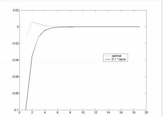
∆ are very small, implying that commodity price intervention yields extremely modest welfare gains by comparison with the adoption of an optimal degree of monetary policy inertia. We also note in Figure 3 (plotted for the already high value of ψ_R =32) that the optimal intervention policy and the naïve policy of complete commodity price stabilization correspond to radically different trajectories for λ_t.

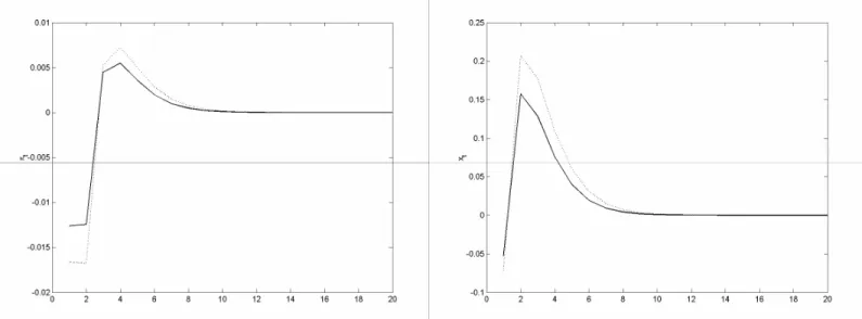
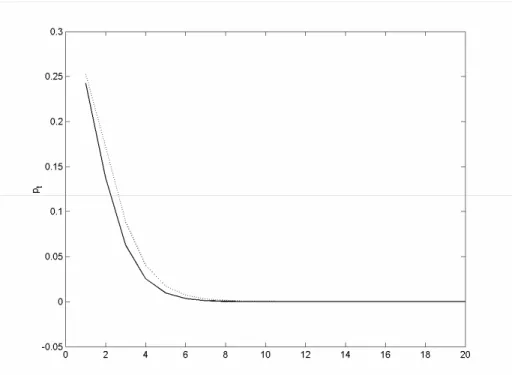
These trajectories differ most notably in the intensity of intervention, optimal intervention being quite weak compared to the naïve policy – so much so that the naïve path of λt had to be scaled down by a factor of 10 for the optimal trajectory to appear clearly in the same plot. Actually, if we were to plot the responses of inflation, interest rates, the output gap and the relative price p_t to an innovation in ε_t according to the optimal plans with and without intervention, the difference between two paths for each variable would barely be discernible. The optimal and the naïve intervention policies differ also in terms of the shape of the response of λ_t. Optimal policy responds to a positive innovation to ε_t (whose effects

Although optimal intervention produces pitiful improvements in terms of welfare, that does not mean that complete stabilization of εt +λt could not produce a significant worsening by comparison to free trade. The values of ∆′ reported in Table 1 are not only negative but are also much larger in absolute value than the values of ∆. If ψ_R is not too large, naïve intervention can cause losses of the same order of magnitude as keeping trade free but reverting all the way back to the class of non-inertial monetary policy rules.

It is important to understand where the case for intervention – even weak as it is – stems from in this economy. Movements in the natural rate of interest require the nominal interest rate to move in order to maintain macroeconomic stability, but that is now costly, and as a result stabilization of inflation and the output gap will not be complete. The natural interest rate incorporates a number of domestic supply and demand shocks, including shocks to government expenditures on goods and services, and also shocks to international commodity prices, which affect potential output. It can be verified that a given trajectory of the natural interest rate elicits the exact same response in terms of intervention regardless of the nature of the components of the natural rate that happen to be moving – proof of this assertion is provided in the Appendix below. Therefore, optimal intervention is not about responding to international commodity price shocks, but about responding to natural rate shocks, whatever their source. In particular, intervention takes place even in response to natural rate variations due exclusively to domestic factors totally unrelated to commodity prices.

Any inefficient supply shocks generated by intervention would be a nuisance if it were optimal in their absence to stabilize completely both inflation and the output gap, which is not the case here thanks to the penalty on interest variability. In this case, intervention is actually beneficial because it produces a slight inefficient shock, which – provided that it is indeed small – allows for a better combination of trajectories for inflation, the output gap and the nominal interest rate, satisfying the constraints imposed by the intertemporal IS and by the Phillips curve. It does so in order to produce a smaller joint loss from those three variables according to [21], and despite the fact – demonstrated in section 4 – that departing from the free-trade path of p_t worsens the total contribution of the price misalignment terms collected inside the square brackets in that equation.