Core inflation in a small transition country: choice of optimal measures

(1)

Core inflation in a small transition country:

choice of optimal measures

Gagik G. Aghajanyan 1

Central Bank of Armenia, Statistics Department

Abstract

Several non-monetary (mainly supply) factors affect prices in the short-run. It is widely acknowledged that in countries (especially countries in transition), where the price level is highly volatile and seasonal, it is not expedient for central banks to use official inflation index while formulating monetary policy. For this reason, it is crucial for central banks to work out, study and follow the behavior of core inflation that enables to reflect long-run price movements. This paper presents the application of various methods of calculating core inflation to Armenian data (for 1996:1-2002:12). Each measure is calculated at monthly frequencies and evaluated by different criteria. The analysis shows that core inflation indices, calculated by trimming the distribution of prices at 10 or 15%, are the best and most effective indicators for monetary policy-makers in Armenia, since they capture inflation trends and are closely tied to monetary aggregates. However, the median seems to be the best predictor for forecasting inflation of all core inflation measures discussed in this paper.

JEL Classification: P2, P3, E31, R5

Keywords: inflation, transition country, Armenia

1. Introduction

Ever since the middle of the last century, the central banks started to play a key role in the process of the aggregate demand management. In that context, they tried to manage economic growth, unemployment, wages etc. Only after the breakdown of the Bretton-Woods monetary system the central banks’ key role was realized mainly through the maintenance of the price stability. In line with the development of financial and capital markets the concept of the price stability was also developed and the idea of direct inflation targeting became widespread. This is because the maintenance of price stability creates conditions for households and businesses to formulate healthy

1_Contact:_{a.gagik@cba.am}_{The author gratefully acknowledges that this research has been funded by the}

(2)

expectations on price movements and make right decisions on consumption and investments.

Since 1996 the law “On the Central Bank of the Republic of Armenia” made the maintenance of price stability the main goal of the Central Bank of the Republic of Armenia (CBA). In the annual monetary policy program CBA announces the appropriate annual rate of inflation, and describes the main policy measures needed for keeping the inflation within the determined level.

However, these developments brought many difficulties and raised peculiarities that central banks need to explain when they accept inflation targeting as a monetary strategy. The latter refers to such issues as which price indices to choose, how to define them, how to communicate with the public regarding the chosen goal and how to explain deviations from it without confusing it.

Inflation targets were originally expressed in terms of the rate of change or the level of the consumer price index. The consumer price index (CPI) is a weighted average index, representing movements of overall price level, i.e., cost of consumer basket of goods and services, which is measured by the National Statistical Service of the Republic of Armenia (NSS). CPI is highly volatile, due to the seasonality of the production of some goods and services such as agricultural products, and tourism, and to annual cycles of consumer expenditures. The CPI can be treated as a least variance estimator of economy-wide price changes only if the price change distribution is normal (see, e.g. Rae, 1993, Ball and Mankiw, 1995, Jaramillo, 1997).

If the target of monetary authorities is to maintain price stability in the economy, they ought to be able to distinguish between temporary shocks to the price level and a persistent drift of prices. Different shocks like seasonality, crop failures or other short-term fluctuations are beyond the control of monetary authorities. Therefore, central banks should disregard various one-off shocks coming from the supply side and govern or control long-term movements in prices that reflect aggregate demand. While implementing monetary policy, the central bank should react to price changes when there are long-term movements in prices. Sustainable and substantial increases in the price level caused by specific factors mentioned above may lead to the corresponding reaction of the central bank to tighten its monetary policy, which could hurt the whole economy by depressing aggregate demand.

Thus, there is a need for central banks to develop and work out an inflation index that enables them to define and measure inflation for purposes of monetary policy formulation, communication and accountability, and to study and follow its behavior. It should provide the best fit to the trends and movements of the price level. Moreover, as monetary policy affects inflation with a lag, central banks are concerned with the

behavior of future inflation2_{: the index should therefore be forward looking and serve as}

a leading predictor in the process of inflation forecasting. Finally, if a strong relationship between monetary aggregates and the index can be found, this will enable the CBA to use the latter as a target parameter for monetary policy. Monetary policy instruments have an indirect influence on inflation through the corresponding transmission mechanism. Therefore, as Johnson (1999) mentions, policy makers focus on measures of inflation, which abstract from short-term fluctuations in prices. In this case the chosen index of inflation can serve as the much better than CPI indicator of the

2_{As Johnson, 1999, mentions, the most “...useful measures of core inflation will minimize misleading}

(3)

effectiveness of monetary measures taken by CBA in maintaining price stability in Armenia.

The private sector also needs an index, which measures inflation trends, for adjusting sales prices, salaries, interest rates and so on. In other words, such an index serves as an anticipated level of inflation trend, which should be taken into account while concluding contracts or adjusting current activities.

The inflation index, that corresponds to the above mentioned concept and is generally associated with expectations and demand pressure components, is called the core inflation index, or underlying inflation (see, e.g. Alvarez, 1999), trend inflation (see Wozniak, 1999), long-run inflation, or demand-driven inflation (see Apel, 1999). Core inflation expresses general trends of inflation as a persistent or durable component of inflation (see Wyenne, 1999). As is the convention in economic theory, core inflation shows long-term price movements. Johnson (1999) also mentions that core inflation measures “...the general increase in prices” 3_.

The basic idea of core inflation is to calculate a modified rate of inflation, which minimizes the effects of the components subject to relatively strong price fluctuations. In other words, core inflation characterizes long-run equilibrium in the national economy (see Garganas and Simos, 1998). Under conditions of such equilibrium, when the aggregate demand equals the aggregate supply and there are no cyclical fluctuations, core inflation expresses inflationary expectations and is a result of the long-run influence of fundamental factors.

Roger (1998) tries to distinguish persistent and transient parts of inflation. Supply-driven relative price changes are treated as factors that have transient influence on aggregate inflation rate, and he suggests that core inflation is connected with expectations and demand factors of inflation. He considers two concepts of core inflation, a persistent component of inflation and as a generalized component of inflation. The first concept is based on the statement of Milton Friedman that inflation

is a monetary phenomenon4. The persistency of core inflation implies also its low

volatility. The second concept focuses on the notion that if the increase in relative prices of some goods is not offset by the reduction of relative prices of other goods, then core

inflation shows “the generality of movements in prices”5_{. However, as Cutler (2001)}

mentions, in the short run movements of relative prices may not offset each other, and relative prices are therefore likely to affect aggregate inflation.

Thus, core inflation is free from the influence of seasonal and random factors, and is characterized as a time-series with low variability. It has also high persistence of its time-series values and slow-changing trend (see Garganas and Simos, 1998).

Nowadays core inflation indices are calculated in many countries and used in macroeconomic policy decision-making. As a rule, central banks, and not statistical

agencies, compile and use core inflation indices6_{. Thus, central banks of England,}

Canada, USA, Greece, Spain, Italy, Belgium, Netherlands, Sweden, Finland, Poland, India, Japan, Australia, New Zealand and some other countries calculate and monitor core inflation on a periodical basis. Some countries use core inflation as a final target

(4)

(e.g., the Bank of Thailand, Monetary Policy Committee in the UK7) or operational

target (e.g., the Bank of Canada8_{) for monetary policy.}

Since 1996 CBA started to calculate a core inflation index and apply it for limited analytical purposes. The calculation is based on the exclusion of prices of seasonal goods (fruits and vegetables) and administered services whose tariffs are regulated by the government. However, this method has some disadvantages. First, part of price changes of seasonal goods and administered services may be caused by monetary factors, and this part should not be eliminated from the calculations. Moreover, seasonality is determined as a seasonality of production, and fluctuations of prices are not taken into account. Thus, CBA needs to develop the methods of core inflation measurement in order to find the measure that fits the best to monetary policy requirements.

At the same time there are drawbacks that impede the calculation and use of core inflation by policy-makers in Armenia. First, the issue of the proper distinction between supply and demand shocks. In Armenia the process of revealing and estimating supply and demand shocks is complicated by several obstacles, in particular by the high level of the shadow (unobserved) economy and dollarization. According to official data, more than 30% of GDP is produced in the shadow economy. As for the dollarization level, the ratio of deposits in foreign currency in overall deposits amounts to

approximately 70% of total deposits, or 40% of the money supply9_{. In addition there are}

huge quantities of foreign currencies that circulate as cash in the economy, but are not included in the recorded money supply. In such conditions official data on aggregate supply and demand deviate from actual levels of production and consumption, and official measure of money supply do not reflect the actual quantity of money in circulation. Thus, the estimation of supply and demand shocks seems not to be too precise.

Second, it is very difficult to determine and filter out transitory changes in prices. Temporary fluctuations may easily be confused with permanent changes of prices. Moreover, changes that have been taken as permanent and included in core inflation proved ex post to be only temporary.

Policy-makers should also distinguish sector specific shocks from aggregate shocks (see Cutler, 2001). Monetary authorities are supposed to react to the latter shocks, since the inflation expresses the change of aggregate price level. It should be also noted, that if substantial adverse supply shocks (most probably with long-run effects) take place in a country, and the central bank doesn’t take them into account and react to them, they may lead to considerable economic recessions. Such an event occurred during the 90’s, when while the Soviet economy was collapsing, prices were liberalized and exchange rates were depreciated, the central banks of Armenia and other CIS countries reduced substantially real money supplies in circulation in order to curb inflation. In this struggle with hyperinflation, the actions of monetary authorities brought about the decline of economic activity and the development of arrears in national economies.

Finally, if Armenia, a small and open economy, is treated as price-taker, then the influence of international prices and exchange rates on domestic prices is substantial and should be taken into account by policy-makers.

7_{Cutler, 2001, p.4.} 8_{Johnson, 1999, p. 8.}

(5)

2. Inflation in Armenia

CPI changes in Armenia are caused not only by monetary but also non-monetary factors such as fiscal policy, structural shifts in the economy, exchange rate and import prices movements, climate changes, real sector shocks, etc. The influence of these non-monetary factors makes CPI changes highly volatile and uncontrollable by the CBA. Thus droughts in 2000 and 2002 significantly influenced on prices and pushed them up. Besides that, the CPI in the Republic of Armenia is characterized by extreme

seasonal fluctuations10_{. Moreover, the high weight of irregular components, which for}

price indices of beverages, tobacco, medical goods and services composed more than 50% in 1995-2002, complicates inflation forecasting.

The CPI in Armenia is calculated on the basis of constant weights of goods and services included in a consumer basket, as an average weighted price index (Laspeyres formula):

∑

= =

= _K

i i i K

i

i t i i i t

q p

p p q p C P I

1 0 0

1 0

0 0

pi 0_{, p}

i

1 _{- individual price levels of item}_i_{in base period (}₀_{) and current period (}_t_),

qi 0

– volume of consumption of individual item i in base period,

K – the total number of items in the basket, equals 400.

The CPI formula can be presented in terms of weights and individual price indices:

*

t t

i i

CPI =

∑

w π (2)

wi – individual weight of item i in consumer basket in base period π_it

– individual price index of item i for current period (month) t

Weights wi in formula (2) are defined as

11

∑

=

400

i i i

i i

i _p _q

q p

w

1 0 0

0 0

The NSS conducts annual household budget surveys for re-weighting the consumer basket. The changes in the structure of consumer basket for the period of 1993-2003 are presented in Figure 1.

10_{According to CBA calculations, in recent years the share of seasonal components in CPI variance was}

about 80%. Calculations have been based on figures of the NSS. The decomposition of the variance of

time-series is done by the following formula:

∑

= =

′ − +

− ′ + − =

− n

i

n

i

i i i

i n

i i n

i

i y y y y y y y

y

1 1

2 2

2

1 1

2

) ~ ( )

~ ~ ( )

~ ( )

( , where yi is an individual monthly

index, y – the average index for the period, ~y_i– trend level, and ~y_i′– trend level adjusted by a seasonal coefficient. Price indices of groups are geometrical means of individual price indices of goods in the group..

11_{Note, that weights}_w

i, calculated based on (t-1) year information, are constant for all months of current year. Thus, by calculating monthly CPI, NSS changes only price indices πit in the formula (2).

(1)

(6)

Figure 1. Structure of consumer basket, 1993 - 2003.

0% 20% 40% 60% 80% 100%

1993 1994 1995 1996 1997 1998 1999 2000 2001 2002 2003

Foods Non-foods Services

Source: NSS data.

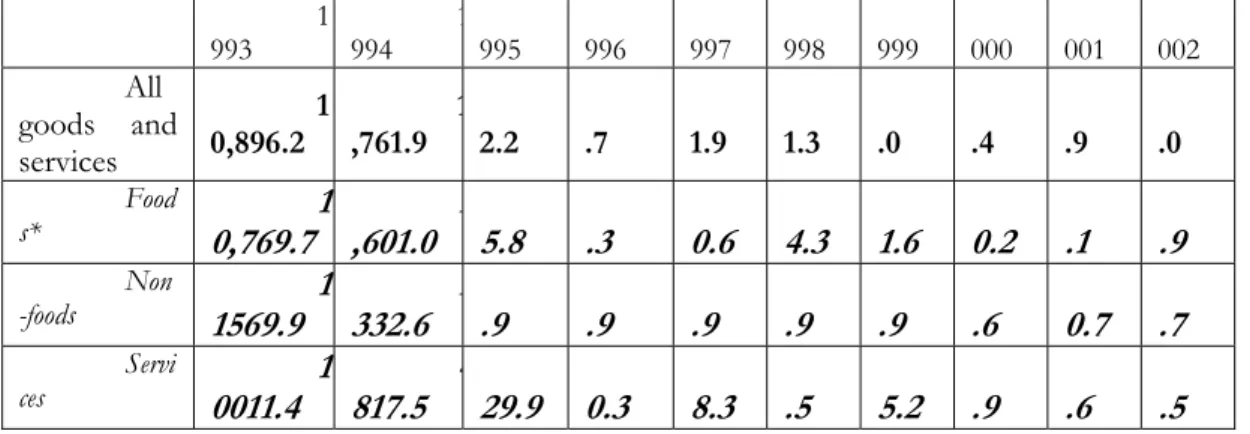
During transition, a substantial stabilization of inflation processes was observable in Armenia. In particular, the inflation rate fell down from 1761.9% in 1994 to 2.0% in 2002 (Table 1).

Table 1. Inflation rates in the Republic of Armenia, as compared to December of previous year 1

993

1

994 995 996 997 998 999 000 001 002

All goods and services

1 0,896.2

1

,761.9 2.2 .7 1.9 1.3 .0 .4 .9 .0

Food

s* _0,769.71 _{,601.0 5.8 .3 0.6 4.3 1.6 0.2 .1 .9}1

Non

-foods _1569.91 _{332.6 .9 .9 .9 .9 .9 .6 0.7 .7}1 Servi

ces _0011.41 _{817.5 29.9}4 _{0.3 8.3 .5 5.2 .9 .6 .5}

*included alcoholic beverages and tobacco Source: NSS data.

The price stabilization was accompanied by continuing price liberalization and implementation of reforms in the tax system, e.g., increases of the tax rates and improved tax administration. Although these processes have nearly come to the end in 1998, real appreciation of the Armenian dram against the Russian ruble, which took place in the aftermath of the financial crisis in Russia, led to a large inflow of cheap imports, which in turn resulted in the reduction of prices. The reduction of remittances and transfers inflowing from Russia was another spillover effect of this crisis.

(7)

from 1999 smoothed (centered 13-point moving averages)12_{monthly inflation rates}

fluctuate around 0% level (Figure 2).

Figure 2. Monthly inflation rates, 1995 - 2002.

-6 -4 -2 0 2 4 6 8

Jan-95 Jan-96 Jan-97 Jan-98 Jan-99 Jan-00 Jan-01 Jan-02

Official inflation, % Smoothed inflation, %

Source: official inflation – NSS data, smoothed inflation – CBA..

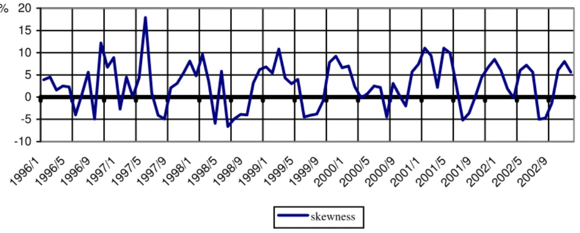
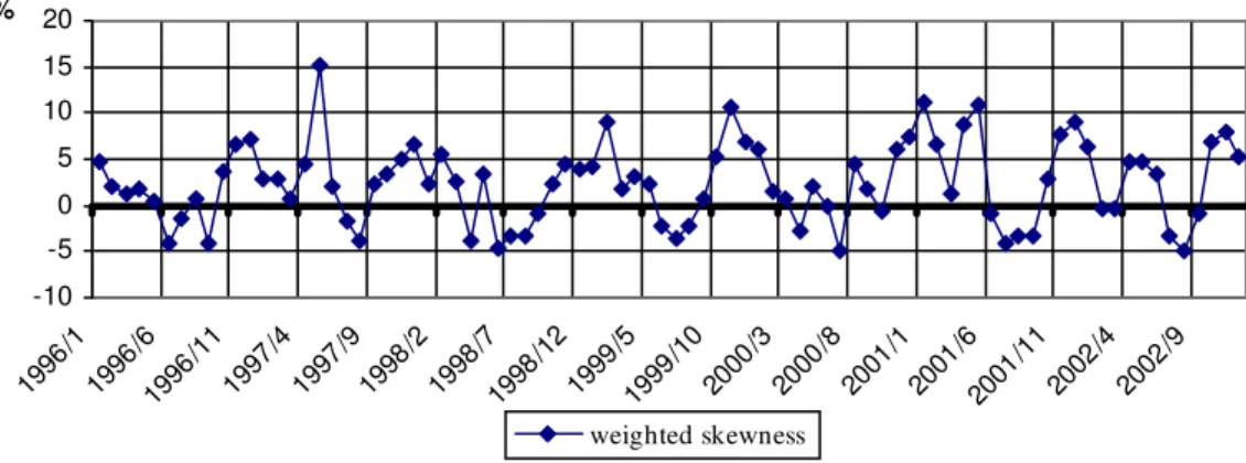
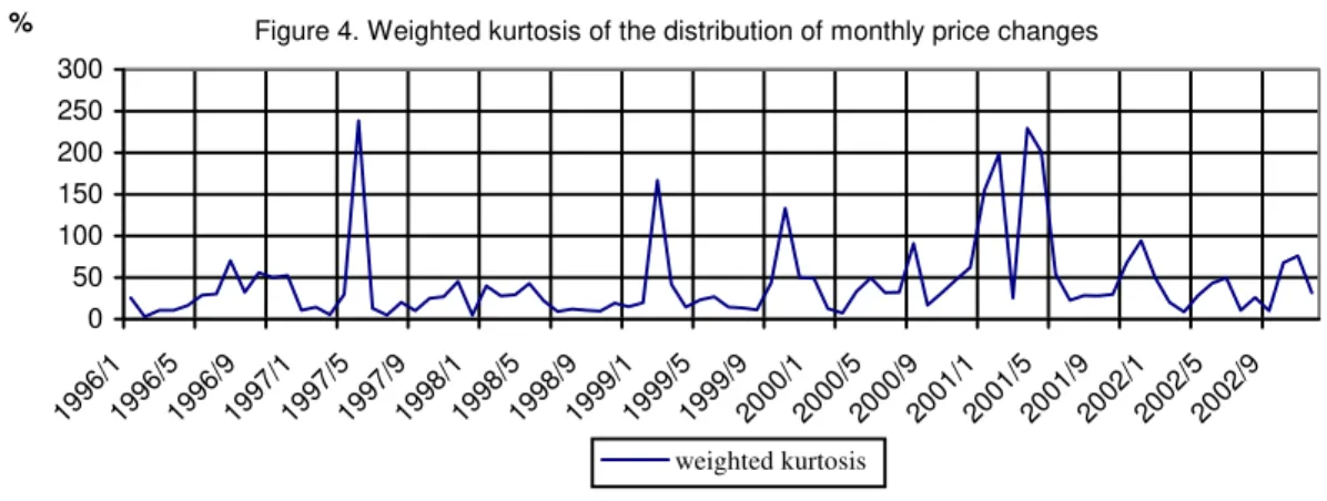
During a year the CPI increases and falls mainly due to seasonal fluctuations of prices of fruits and vegetables. In 1996-2002 the coefficient of variation was relatively stable and composed 8.1% for unweighted and 9% for weighted mean and standard

deviation indices. On the other hand, skewness and kurtosis13_{deviate significantly from}

normal distribution (see Appendix 1). Moreover, in the majority of cases (73% for weighted and 70% for unweighted skewness) the actual levels of skewness were positive (“right-side” distribution of price indices), and at the same time, the actual kurtosis was too high (“leptokurtic” distribution of price indices).

Thus, the time-series of both CPI and its components are too volatile and their

distributions diverge from normal14. Therefore, the use of CPI for the purpose of

formulating and implementing monetary policy may result in inadequate reaction of the CBA to price movements and diminish the effectiveness of aggregate demand management. Hence, for policy purposes CBA needs to calculate and elaborate an appropriate core inflation index.

3. Measures of core inflation

A number of methods or techniques of core inflation measurement can be found in economic literature. Their measurement methods are classified in different groups by different researchers (see, e.g., Roger, 1998; Core inflation rates as a tool of price analysis, 2000; Wozniak, 1999; Cutler, 2001; Kearns, 1998; Clark, 2001; Johnson, 1999, Cockerell, 1999). The methods have been classified into three main groups: (i)

12_{The smoothed levels are calculated by the following formula:}

12

2 1 2

1

6 5 4 3 2 1 1

2 3 4 5

6 − − − − − + + + + + +

− + + + + + + + + + + + +

= t t t t t t t t t t t t t

sm t

π π π π π π π π π π π π π π

13_{Skewness and kurtosis (both unweighted and weighted) have been calculated in accordance of formulas}

presented in Bryan, 1996.

14_{As Roger, 2000, mentions, in case of high kurtosis and right skewness other estimators of inflation (i.e.,}

(8)

exclusion, (ii) statistical and (iii) econometric methods. For exclusion and statistical methods, researchers design core inflation by removing those price indices that express high volatility (at a point of time or over some period of time), which they treated as

“non-representative or idiosyncratic movements15_{”. Econometric methods allow the}

modeling of inflation, i.e., measuring core inflation based on the interrelationship between prices and other economic indicators.

In exclusion-based methods, or methods from the “central-bank view” (see Apel, 1999), (1) price changes of some goods and services, or (2) the impact of some macroeconomic indicators or administrative measures on prices, are excluded.

The impact of macroeconomic indicators may substantially distort the main direction of price movements. Thus, some central banks (for instance, the central banks of New Zealand, Finland, Canada, England, Sweden) estimate and isolate the influence of indirect taxes, subsidies, various government levies, and international prices as well as exchange rate movements on the price level (see, e.g., Roger, 1998). However, such an adjustment of price movements has its disadvantages. First, the above mentioned factors compose only part of the supply factors that influence the price level. As Roger (1998) mentions, price wars between competitors or the uncontrollable behavior of monopolists have the same effect on prices and should also be considered for exclusion. However, because of the above mentioned drawbacks, the impact of macroeconomic variables or administrative measures on prices in Armenia has not been eliminated in the calculated core inflation.

The exclusion of price changes of some goods and services is conditioned on the fact that (a) those goods and services are seasonal or “primarily

supply-determined”16_{or that (b) price movements of some goods and services are thought to}

be volatile enough to obscure long-term movements of inflation. Basically, the choice of items to exclude depends on the points of view of many central bankers, regarding core inflation “…as the aggregate inflation excluding a variety of items whose price movements are deemed likely to distort or obscure the more general trend of other

prices”17. Some countries exclude, for instance, food and energy, government charges,

interest costs, and rents from the consumer basket in the calculation of the core inflation index (see, e.g., Core inflation rates as a tool of price analysis, 2000; Wozniak, 1999; Cecchetti, 1997, Cutler, 2001). The exclusion of prices of some goods (like

seasonal foods in Thailand, seasonal and non-seasonal foods in the USA18) is stipulated

by the seasonality of the production of those goods. The price movements of other goods (e.g., energy) proved primarily to be the result of supply shocks. Finally, some kinds of goods and services (like electricity or phone charges in Armenia, tobacco or

alcohol in Poland19) are excluded from calculations due to the fact that their prices are

determined or regulated by the government.

Starting from 1996 the CBA has calculated a core inflation index based on the

exclusion of seasonal goods (fruits and vegetables) and administered services20_{. During}

1996-2002 seasonal goods and administered services composed 18% of consumer

15_{Johnson, 1999, p. 7.} 16_{Roger, 1998, p. 19.} 17_{Roger, 1998, p. 4.} 18_{Cutler, 2001, p. 12.} 19_{Wozniak, 1999, p. 43.}

20_{Electricity, water, natural gas, bus, metro, phone charges and some other services, which tariffs are}

(9)

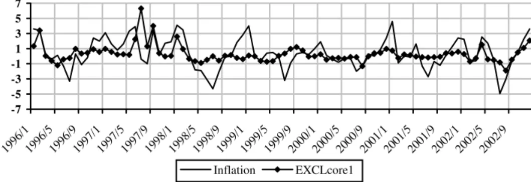
basket in average. Despite the elimination of seasonal goods and administered services,

the calculated inflation measure (EXCLcore1, month to month)21_{still remains volatile.}

In the middle of 1997 and the beginning of 1998 the high level of core inflation is explained mainly by changes of indirect taxes and government levies, the acceleration of core inflation in the second half of 2002 is due basically by the pressure of growing consumer expenditures.

However, while excluding some individual prices, the seasonality of goods is determined by a seasonality of production, and fluctuations of prices are not taken into account. Therefore, another two exclusion methods have been applied for getting rid off the volatility of price movements. The exclusion of highly volatile items is widely discussed in the economic literature (see, e.g., Wozniak, 1999; Johnson, 1999; Core inflation rates as a tool of price analysis, 2000). While excluding highly volatile items, the following issues should be precisely defined: (a) the time horizon, over which volatility is to be investigated, (b) the measure of volatility, and (c) the minimum level of volatility, above which items, having higher volatility, are supposed to be excluded.

For Armenian data the period from 1996 to 2002 has been chosen as a time horizon. Two measures of volatility have been chosen: the coefficient of variation and the standard deviation.

The individual coefficients of variation22_{have been calculated for annual price}

changes of all items (for every year in the above period). Based on the previous year coefficients of variation as a measure of volatility, prices of those goods and services have been excluded that have had a coefficient of variation (in the previous year) higher than the average level of individual coefficients of variation. The weighted mean of price

changes of the remaining items shows core inflation (EXCLcore2)23. It should also be

mentioned that in 1996 40% of the consumer basket were excluded from the calculation of the core inflation, in 2002 – only 20%.

For the application of the standard deviation as a measure of volatility monthly standard deviations of price changes of all items were calculated. Those goods and services were excluded whose absolute price indices exceeded monthly inflation plus 1.5 standard deviations. The excluded items are treated as outliers. This price index has been designated the core inflation index (EXCLcore3). On average, during 1996-2002, 6-8% of the consumer basket was eliminated from the calculations.

The exclusion methods have several disadvantages. The exclusion of some components presupposes that price fluctuations are non-monetary and do not contain information relevant to the long-term price trend. However, irregular component may have supply or demand nature. As a result, the mean price level calculated without excluded items may give a biased estimate of the general price movements. Besides, the influence of various non-monetary shocks still exists in price movements of remaining goods and services.

The second group – the statistical approach – comprises methods that are

used to decrease the volatility of price movements, i.e. the variance of CPI. Thus, fluctuations of CPI are subject to the adjustment by using various statistical methods. The need to apply statistical methods is stipulated by the fact that consumer price changes proved to be highly kurtotic. Thus, the distribution of price changes deviates

21_{Some calculated core inflation measures are presented in Appendix 2.}

22_{The coefficient of variation equals the standard deviation divided by the mean.}

23_{While designing 12-month EXCLcore2 figures for 1996 have not been calculated due to substantial}

(10)

from normal distribution and CPI is not an efficient indicator of the inflation trend. The methods of median, weighted median, trimmed means, double weighted and smoothing (Hodrick-Prescott) measures are widely discussed in the literature and have been calculated within this research.

The median reflects the price change of the item that divides the ordered distribution of individual price indices into equal parts. Bryan and Pike (1991) have found it a “more robust measure on central tendency” than CPI. As is shown in Appendix 2, in Armenia the volatility of both measures of the median (MED for the change over the previous month and MED (12) for that over same month of the previous year) is too low.

The weighted median allows us to pick the price index of the item that corresponds

to the half of the cumulative weight of the distribution.24_{Bryan and Cecchetti (1994)}

consider the weighted median as highly appropriate for forecasting inflation. Cutler (2001) calls individual inflation rates, which are excluded while applying weighted-median or trimmed means methods, as inflation outliers. In all cases the usefulness of this method depends on the distribution of price changes: if the distribution deviates from normal, then the weighted median is supposed to show the inflation trend more precisely than the weighted mean. In Armenia the weighted median expresses higher variability in comparison with the simple median measure of core inflation.

Trimmed means are calculated by trimming some part from the tails of the ordered distribution of individual price changes, and re-weighting the remainder. The rationale here is that when a substantial supply or demand shock takes place and influences the prices of some goods or services, indices of those goods or services stretch and skew the overall distribution. In this case the arithmetic mean, weighted according to consumer basket, doesn’t show the general price trend. So the distribution has to be trimmed. Another way to explain this, is that outlying individual price indices may

reflect relative price changes but have no effect on inflation in the long run25_.

If the distribution of individual price indices is skewed, then trimming will change the mean. The most important issue to be decided while applying this method is a determination of the best trim or cut-off level. Many researchers, all of whom have failed either to yield a clear-cut result or to be regarded as uncontroversial, have developed various optimization methods. Bryan, Cecchetti and Wiggins (1997) have found the 10% trimmed mean the most appropriate estimator of core inflation for US figures. Jaramillo (1998) has calculated the optimal (asymmetric) trimmed means for Colombian figures: 12% is trimmed from the upper and 24% from the lower tail. The Bank of England regularly calculates a 15% trimmed mean and publishes in the Bank’s “Inflation Report”. Wozniak (1999) has also calculated standard deviation trimmed means, based on the volatility of price changes rather than individual weights in the consumer basket.

In the case of Armenian data the distribution of individual monthly price indices has been ordered from the lowest index to the highest. Then some percent of the number of these price indices was removed from both tails. When the distribution is

trimmed by α% from both tails, then the trimmed mean xα(t) can be defined as

24_{For the calculation of the weighted median the monthly distribution of individual price changes is}

ordered from the lowest to the highest, the index of the item whose cumulative weight reaches 50% is taken as an indicator of core inflation.

(11)

∑

∈

− =

α

α α

I i

i ix t

w t

x ( )

100 2 1

1 )

( 26

(4)

where Iα is the set of price changes that is included in the calculation of core

inflation, i.e., the collection of price changes whose cumulative weights lies between

α/100 and (1-α/100). It should also be noted that if α= 0, then the trimmed mean is

actually identical with the official inflation, and when α=50 the trimmed mean coincides

with the weighted-median of the cross-section distribution of price changes. The

statistical theory does not give any guidance for the choice of the optimal level of α. The

following values of α have been applied in this research: 5, 10, 15, 20, 25, 30, 35, 40, and

45. Time-series of trimmed means for α=10 and 40% are presented in Appendix 2. The

higher the level of α, the closer does core inflation tend to the trend of inflation

The shortcoming of this method is that over the observation period prices of some goods or services can demonstrate a declining or increasing trend because of technical progress, quality changes and so on. For instance prices of data-processing goods and telephones in Germany (Core inflation rates as a tool of price analysis, 2000) show a declining trend which has nothing to do with transitory price movements. The exclusion of the price indices of such goods and services can bias (usually upward) the calculated core inflation.

The double weighted measure assumes the process of double-weighting of official weights by the reciprocal of the standard deviation of the difference between individual price changes and total CPI (see, e.g., Johnson, 1999). Thus, the greater the difference, the smaller is the weight. The rationale here is that not all large changes in prices should be treated as noisy or transient changes, and all components of the consumer basket are to participate in the designed core inflation. An alternative suggestion is to weigh price changes of goods and services by their ability to predict (estimate) future levels of inflation (see Blinder, 1997). Its essence is to make statistical processing of individual

price changes and eliminate those, which are too volatile27. The double-weighted

measure for Armenian data has been calculated by the following formula:

∑

=

= n

i

it itdwt

DW 1

π (5)

Where dwtit is the double weight, calculated by multiplying the weight of the item

i in the consumer basket (wi) by the inverse of the standard deviation (σi) of the

difference between the price change of the item (πit) and the CPI (πt

cpi

) in twelve months (t) of the previous year:

∑

=

= _n

i i

i i i it

w w dwt

1

1 1

σ σ

,

[

]

2

1 12

1

2 ) (

) (

1 1

⎥ ⎦ ⎤ ⎢

⎣ ⎡

− − −

−

=

∑

= t

cpi t it cpi t it i

n π π π π

σ (6)

n – quantity of items in consumer basket

One can list the following disadvantages of this method: (a) as a core inflation index may be chosen a price index of random good or service, (b) the price of that good or service can fluctuate under non-monetary factors, (c) in case of biased (not normal)

(12)

distribution of individual prices the results also can be biased, (d) this statistical measure of core inflation is difficult to explain to the public and to model with other economic indicators. It should also be noted that by applying the previous year’s levels of standard deviation we impose tendencies of the previous year on the current one. Thus, it seems that an additional research is needed. In particular, two alternative approaches may be suggested for the calculation of standard deviations: (1) the use of long historical periods; (2) the use of the last 12 months data for each month.

From the range of smoothing methods the Hodrick-Prescott filter has been applied

to Armenian data. It should be mentioned that the Hodrick-Prescott filter is widely used in the extraction of trends of time series (see, e.g. Meyler, 1999). It is known from the theory of statistics that the degree of smoothness of time-series depends on the level of

a smoothing parameter λ. Despite the fact, that for monthly time-series it is

recommended to use λ=14400, for Armenian data following levels of λ have been also

used: 50, 100, 500, 1000, 5000 and 10000.

Finally, the third group – the econometric approach – includes vector auto

regression (VAR) modeling and the Dynamic Factor Index (see, e.g., Quah and Vahey, 1995; Bryan and Cecchetti, 1993; Fase and Folkertsma, 1996; Gartner and Wehinger, 1998; Garganas and Simos, 1998). The rationale is to derive a measure of core inflation using the long-run neutrality assumption of monetary theory. In other words, such methods, which Roger (1998) calls “multivariate methods”, distinguish between core inflation that is neutral to medium- or long-run changes of output, and non-core inflation or residual elements that are associated with persistent effects of output. However, for countries in transition most econometric methods have a very limited scope of application. First, there are problems with data quality and consistency. Second, econometric methods require long time-series. Third, countries in transition are characterized by rapid structural changes, which make it impossible to use most econometric methods. Hence neither VAR modeling nor Dynamic Factor Index have been applied in the context of the present research.

As a development of core inflation research in Armenia following directions are quite visible: (1) the application of asymmetric trimming, and (2) the application of factor analysis.

4. Choice of optimal measure of core inflation

Two criteria should guide the choice of the best measure of core inflation: Movements of core inflation should express inflation tendencies. A strong correlation with official inflation enables the use of core inflation as a predictor for the forecast of future inflation.

Core inflation should display a strong relationship to monetary aggregates. This enables monetary authorities to find the measure that could be regulated by monetary policy-makers. In other words, when monetary authorities focus on the persistent trends in inflation, core inflation becomes “... a measure of the inflation which is the outcome of policy28”.

For policy-makers core inflation can be treated as a tool for economic policy. One of the best applications of core inflation is its use as an inflation target. While choosing an inflation target, the candidate core inflation measure should satisfy several

(13)

requirements. Thus, the measure of core inflation with the best approximation to inflation trends and the strongest measure of ex ante control, i.e., a strong correlation with monetary aggregates, can serve as an inflation target for monetary policy, since it is less volatile than official inflation and will enable to minimize the variability of monetary policy instruments (see, e.g., Roger, 1998; Johnson, 1999). On the other hand, Cutler (2001) mentions that if there is an inflation target in a country, the monetary authority, responsible for price stability, should find a core inflation measure which is correlated with targeted inflation and can also serve as an inflation predictor (leading indicator) while forecasting the targeted inflation.

To select the optimal measure of core inflation, we need efficiency criteria. There is no single criterion by which the accuracy of core inflation measurement process can be assessed. Different approaches to evaluate core inflation measures have been presented and widely discussed in the economic literature. I follow Roger (1998), who proposes the following properties or features of core inflation measures: (a) robustness, which implies the ability to distinguish precisely between persistent and transient movements in inflation, (b) unbiasedness, i.e., that core inflation should not be significantly biased relative to the target measure of inflation; in other words, the average levels of core inflation and official CPI inflation should be equal over the long run, (c) timeliness, i.e., the measure of core inflation should be available currently to policymakers to undertake the appropriate measures, (d) credibility—the core inflation index should be externally verifiable.

In this research we use the following measures to operationalize these efficiency criteria:

the minimum root mean square error (RMSE) and the mean absolute deviation (MAD) (see, e.g.,Bryan et al, 1997; Wozniak, 1999)29_,

the maximum correlation with monetary aggregates (see, e.g., Bryan and Cecchetti, 1999; Johnson, 1999),

the maximum correlation with future inflation (see, e.g., Bryan and Cecchetti, 1999; Johnson, 1999).

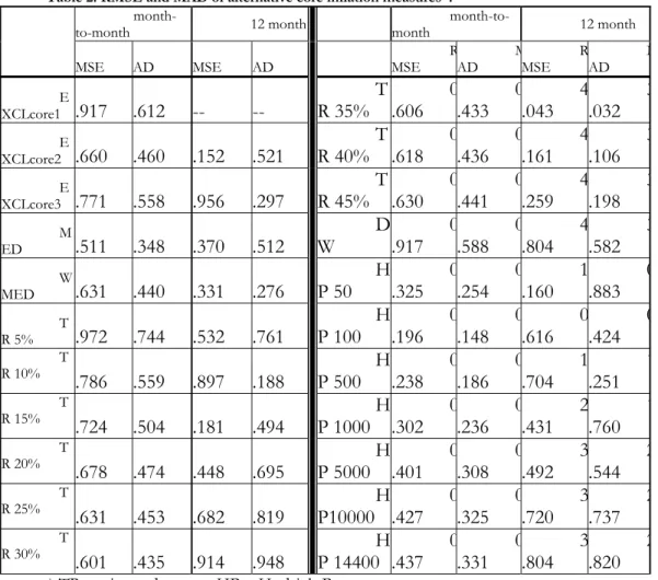
In the application of RMSE and MAD the centered moving average serves as a benchmark inflation: for instance, Bryan and Cecchetti (1997) find 36-month moving average of actual CPI time-series as the best approximation of the trend inflation of the USA, while Wozniak (1999) finds the 24-month measure for Polish data. The rationale for using RMSE and MAD is that if core inflation expresses the main tendencies of inflation, it should be as close as possible to the trend of inflation.

For Armenian data smoothed, centered, 13-point moving averages levels of official inflation, presented in Section 2 above, have been chosen as benchmark inflation. The data presented in Table 2 indicate that core inflation indices, calculated by Hodrick-Prescott filter, provide the best correspondence to inflation trends. It needs to be remembered, however, that the core inflation measure that is closely related to inflation trends, need not be closely tied to monetary policy actions. Thus, RMSE and MAD are necessary but insufficient criteria for making the final decision: other criteria should also be investigated.

29

∑

=

= N

i i

x N RMSE

1 2 ) ( 1

,

∑

=

= N

i i

x N MAD

1 ) ( 1

, where x_i is the difference between core inflation

(14)

Table 2. RMSE and MAD of alternative core inflation measures*.

month-to-month 12 month

MSE AD

R

MSE AD

R MSE M AD R MSE M AD E

XCLcore1 .917 .612 -- --

T R 35% 0 .606 0 .433 4 .043 3 .032 E

XCLcore2 .660 .460

4 .152 .521 T R 40% 0 .618 0 .436 4 .161 3 .106 E

XCLcore3 .771 .558

2 .956 .297 T R 45% 0 .630 0 .441 4 .259 3 .198 M

ED .511 .348

4 .370 .512 D W 0 .917 0 .588 4 .804 3 .582 W

MED .631 .440

4 .331 .276 H P 50 0 .325 0 .254 1 .160 0 .883 T

R 5% .972 .744

2 .532 .761 H P 100 0 .196 0 .148 0 .616 0 .424 T

R 10% _{.786 .559}_{.897 .188}2 _{P 500} H_.238 0_.186 0_.704 1_.251 1

T R 15% .724 .504 3 .181 .494 H P 1000 0 .302 0 .236 2 .431 1 .760 T R 20% .678 .474 3 .448 .695 H P 5000 0 .401 0 .308 3 .492 2 .544 T R 25% .631 .453 3 .682 .819 H P10000 0 .427 0 .325 3 .720 2 .737 T

R 30% _{.601 .435}_{.914 .948}3 _{P 14400}H_.437 0_.331 0_.804 3_.820 2

* TR – trimmed means, HP – Hodrick-Prescott

The efficiency of core inflation measures has also been evaluated on the basis of the correlation of core inflation with monetary aggregates and official inflation.

The evaluation of the relationship between core inflation measures and monetary aggregates was done in two steps. In Step 1 simple regressions between core inflation measures and changes of monetary aggregates—currency in circulation, reserve money, credit to economy, broad money, seasonally adjusted (by centered 13-point moving averages) currency in circulation, seasonally adjusted broad money—were done by the following formula: coret =β0+β1MAt−l+εt, where coret is core inflation measure for

period t, MAt-l is the percentage change of the monetary aggregate in period t-l (l=1, 3, 6,

9, 12). In Step 2 the causality between 12-month changes of monetary aggregates and

core inflation measures with significant R2_{is scrutinized by Granger causality tests. As it}

follows from the results of regressions, i.e., values of R2, presented in Appendix 3, there

is an insignificant statistical relationship between monthly changes of the monetary aggregates and core inflation measures. Therefore, core inflation measures, calculated on the monthly basis should not be used for monetary policy purposes. At the same time the relationship between changes of monetary aggregates, such as currency in circulation and reserve money, over a period of 12-months, and core inflation indices is relatively strong. This applies especially to measures, calculated by the Hodrick-Prescott filter, the median and some trimming methods.

(15)

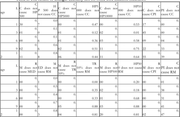
monetary aggregates on alternative measures of core inflation. The test checks for the

lack of causality, hence the lower the probability level reported in the table, the higher the causality between figures. The tests show that the causality between reserve money and core inflation indices is strong, especially for the median and 10 and 15% trimmed means. The relationship between reserve money and CPI is also substantial, but when

we take into account R2_{values (Table 2, Appendix 3), the 12-month median and 10 and}

15% trimmed means are preferable to the CPI as measures of inflation.

Table 3. The results of Granger causality test for some core inflation measures.

L ags

C C does not cause HP 500

H P 500 does not cause CC

C C does not cause HP5000

HP5 000 does not cause CC

C C does not cause HP10000

HP10 000 does not cause CC

C C does not cause CPI

C PI does not cause CC 1 0. 30 0.0 7 0. 00 0.47 0. 00 0.53 0. 17 0. 00 3 0. 01 0.1 0 0. 01 0.12 0. 02 0.01 0. 45 0. 00 6 0. 00 0.1 6 0. 01 0.36 0. 03 0.58 0. 09 0. 04 9 0. 02 0.6 6 0. 02 0.51 0. 11 0.75 0. 22 0. 33 1 2 0. 11 0.8 8 0. 06 0.44 0. 11 0.64 0. 55 0. 39 L ags R M does not cause MED

M ED does not cause RM

R M does not cause TR 10%

TR 10% does not cause RM

R M does not cause HP500

HP50 0 does not cause RM

R M does not cause CPI

C PI does not cause RM 1 0. 00 0.0 1 0. 00 0.00 0. 00 0.20 0. 00 0. 01 3 0. 00 0.5 7 0. 00 0.35 0. 02 0.18 0. 00 0. 38 6 0. 00 0.4 7 0. 00 0.33 0. 01 0.68 0. 00 0. 31 9 0. 00 0.7 8 0. 05 0.88 0. 03 0.88 0. 00 0. 41 1 2 0. 00 0.8 3 0. 04 0.81 0. 20 0.81 0. 02 0. 47

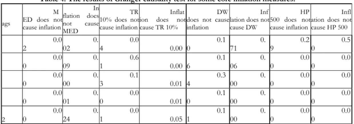
For the evaluation of the relationship between core inflation and official

inflation a two-step evaluation has again been applied30. The results of these calculations

(R2_{), presented in Appendix 4, show that the correlation between monthly core inflation}

measures and monetary aggregates are low, and that they are not efficient predictors for inflation forecasts. As for the 12-month core inflation measures, the statistical relationship with official inflation is substantial for the median and the Hodrick-Prescott

filter. Furthermore, the calculation of the regression coefficient b and the application of

the Wald test31_{show that double-weighted measure (with 6 and 9 lags) and HP 500}

(with 3 lags) seem to perfectly predict official inflation. Finally, from the results of Granger causality test (Table 4) we can conclude that 12-month median core inflation

30_{In Step 1 simple regressions between core inflation and official inflation rates have been realized by the}

following formula: πt=α0+α1coret−l +ut, where πt is the official inflation in period t, coret-l is core inflation measure for period (t-l). Then the issue of to what extent 12-month core inflation measures may be used for forecasting the official inflation has been clarified by calculating regression coefficient b by the following formula (see Cutler, 2001, Johnson, 1999): πt =a+b*coret−l+(1−b)*πt−l+εt. Then Wald test

has been conducted for regression coefficient b. In Step 2 the Granger causality test has been fulfilled to check the results, obtained in Step 1.

31_{The Wald test has been done for those measures that are strongly correlated with official inflation, and}

(16)

(with 3 and 12 lags) turn out to be the best leading indicators for predicting inflation. Thus the median, one of the simplest measures to compute, may be effectively used in inflation and other macroeconomic models.

Table 4. The results of Granger causality test for some core inflation measures.

ags

M ED does not cause inflation

In flation does not cause MED

TR 10% does not cause inflation

Inflat ion does not cause TR 10%

DW does not cause inflation

Inf lation does not cause DW

HP 500 does not cause inflation

Infl ation does not cause HP 500

0.0 2

0. 02

0.0

4 0.00

0.1 0

0. 71

0.2 9

0.5 0

0.0 0

0. 09

0.6

1 0.00

0.1 6

0. 06

0.0 0

0. 00

0.1

3 0.01

0.3 4

0. 00

0.0 0

0. 01

0.0

0 0.01

0.1 0

0. 00

0.0 0

2

0.0 0

0. 24

0.0

1 0.05

0.1 1

0. 00

0.0 0

Taking into account the above-mentioned requirements, 12-month trimmed

means with α=10 or α=15% seem to be the best targets for monetary policy, since they

are closely correlated with monetary aggregates—reserve money in this case—and inflation trends.

It is useful also to note that the final decision on the choice of an inflation target should be based on more detailed and comprehensive analyses of the relationship between monetary actions and price changes in Armenia. Clearly, if the selected inflation target is not the official CPI, which measures the cost of living, it has to be made acceptable and understandable to the public.

On the other hand, the issue of the appropriate reaction of central banks to price movements should be taken into account. Should the central bank react immediately or gradually? To what extent should it at all react? These are questions that are open and require future research.

5. Conclusion

Issues of price stability are of great importance for monetary authorities, especially in countries with inflation targets. The accurate measurement of inflation does therefore assume crucial importance for the policy-makers. The CPI is inappropriate for policy purposes for various reasons. First, it is highly volatile. Next, its distribution of individual price changes is not normal and the CPI therefore turns out to be a biased estimator of inflation tendencies. Core inflation measures are alternatives to the CPI that should not suffer from these defects. Since monetary policy-makers are those who should react to persistent price movements, central banks of several countries calculate and elaborate core inflation measures.

Core inflation expresses the general trends of inflation. In other words, it shows long-term price movements. Thus, its movements are free from the influence of seasonal and random factors and are characterized by low variability.

(17)

double-weighted indices, trimmed indices, and the Hodrick-Prescott filter. The calculated core inflation indices were evaluated by various criteria.

Our findings reveal that monthly core inflation indices are not significantly correlated with either inflation trends or monetary aggregates and future inflation levels. Thus, they should not be used for policy purposes. But core inflation indices calculated by trimming the distribution of prices at 10 or 15% are optimal indicators for monetary policy purposes in Armenia, since they capture inflation trends and are closely tied with monetary aggregates. Monetary policy-makers can treat them as the most controllable or governable inflation measures. The median has been selected as best inflation predictor among all core inflation measures discussed in the paper.

Despite these results, it is obvious that while formulating and implementing monetary policy the CBA should thoroughly analyze the relationship between price changes and other economic variables, and study thoroughly appropriate reactions to price movements.

References

Alvarez, L.J. and M.L. Matea. (1999), ‘Underlying inflation measures in Spain’, BIS, Proceedings of the workshop of central bank model builders

Apel, M. and P. Jansson (1999), ‘A parametric approach for estimating core inflation and inter-preting the inflation process’, BIS, Proceedings of the workshop of central bank model builders

Ball, L. and N.G. Mankiw (1995), ‘Relative price changes as aggregate supply shocks’, Quarterly Journal of Economics, 110, 161-193

Blinder, A.S. (1997), ‘Commentary’, Federal Reserve Bank of St. Louis Review, 79, 157-160

Bryan, M. F. and S.G. Cecchetti. (1993), ‘The Consumer Price Index as a Measure of Inflation’, NBER Working Paper No. 4505.

Bryan, M. F. and S.G. Cecchetti. (1994), ‘Measuring Core Inflation’, in N.G. Mankiw (ed.), Monetary Policy. NBER Studies in Business Cycles, 29, 195-215

Bryan, M. F. and S.G. Cecchetti (1999), ‘The monthly measurement of core inflation in Japan’, Monetary and Economic Studies/May 1999, 77-101

Bryan, M.F., S.G. Cecchetti and R.L. Wiggins. (1997), ‘Efficient inflation estimation’, NBER Working Paper No.6183

Bryan, M. F. and S.G. Cecchetti. (1996), ‘Inflation and the distribution of price changes’, NBER Working Paper No.5793

Bryan, M.F. and C.J. Pike. (1991), ‘Median price changes: an alternative approach to measuring current monetary inflation’, Federal Reserve Bank of Cleveland Economic Commentary, December 1 Cecchetti, S.G. (1997), ‘Measuring short-run inflation for central bankers’, Federal Reserve Bank of

St. Louis Review 79, 143-155

Clark, T.E. (2001), ‘Comparing measures of core inflation’, Federal Reserve Bank of Kansas City, Economic Review, second quarter 2001

Cockerell, L. (1999), ‘Measures of inflation and inflation targeting in Australia’, BIS, Proceedings of the workshop of central bank model builders

‘Core inflation rates as a tool of price analysis’. Deutche Bundesbank Monthly Report, April 2000 Cutler, J. (2001), ‘Core inflation in the UK’, Bank of England External MPC Unit Discussion Paper

(18)

Fase, M. and C.Folkertsma. (1996), ‘Measuring inflation: an attempt to operationalize Carl Menger’s concept of the inner value of money’, De Nederlandsche bank Working Paper

Friedman, M. (1968), ‘Dollars and Deficits’, Prentice-Hall, Englewood Cliffs, N.J.

Garganas, E. and T.Simos. (1998), ‘Techniques for measuring core inflation’, National Bank of Greece Economic and Statistical Bulletin, January 1998, issue 9

Gartner, C. and G.Wehinger. (1998), ‘Core Inflation in Selected European Union Countries’, Oesterreichische Nationalbank Working Paper No. 33, September

Hogan, S., M. Johnson and Th. Lafleche. (2001), ‘Core inflation’, Bank of Canada Technical Report No. 89

Jaramillo, C.F. (1998), ‘Improving the measurement of core inflation in Colombia using asymmetric trimmed means’, Banco de la Republica, Colombia

Johnson M. (1999), ‘Core inflation: a measure of inflation for policy purposes’, BIS, Proceedings of the workshop of central bank model builders

Kearns J. (1998), ‘The distribution and measurement of inflation’, Reserve Bank of Australia Research Discussion Paper 9810

Macklem T. (2001), ‘A new measure of core inflation’, Bank of Canada Review, Autumn 2001 Meyler A. (1999), ‘A Statistical Measure of Core Inflation’, Technical paper no. 2/RT/99, presented

at the 13th Annual Conference of the Irish Economic Association, Westport, Co. Mayo

Quah, D. and S.P. Vahey. (1995), ‘Measuring Core Inflation’, The Economic Journal No. 105

Rae, D. (1993), ‘Are retailers normal? The distribution of consumer price changes in New Zealand’, Discussion Paper G93/7, Reserve Bank of New Zealand, Auckland

Roger, S. (1998), ‘Core inflation: concepts, uses and measurement’, Reserve Bank of New Zealand Discussion Paper G98/9

Roger, S. (2000), ‘Relative prices, Inflation and core inflation’, International Monetary Fund WP/00/58

Wozniak, P. (1999), ‘Various Measures of Underlying Inflation in Poland 1995-1998’, CASE-CEU Working Paper No. 25

Wynne, M.A. (1999), ‘Core Inflation: a Review of Some Conceptual Issues’, BIS, Proceedings of the workshop of central bank model builders

Appendix 1

Figure 1. Skewness of the distribution of monthly price changes

-10 -5 0 5 10 15 20

1996 /1

1996 /5

1996 /9

1997 /1

1997 /5

1997 /9

199 8/1

1998/ 5

1998 /9

1999 /1

1999 /5

1999 /9

2000 /1

2000 /5

200 0/9

2001/ 1

2001 /5

2001 /9

2002 /1

2002 /5

2002 /9

%

(19)

Figure 2. Kurtosis of the distribution of monthly price changes

0 50 100 150 200 250 300 350 400

1996 /1

1996 /6

1996 /11

1997 /4

199 7/9

199 8/2

199 8/7

1998 /12

199 9/5

199 9/10

2000 /3

2000 /8

2001 /1

2001 /6

200 1/11

2002 /4

2002 /9

%

kurtosis

Figure 3. Weighted skew ness of the distribution of monthly price changes

-10 -5 0 5 10 15 20

1996 /1

199 6/6

199 6/11

1997 /4

199 7/9

199 8/2

1998 /7

199 8/12

1999 /5

1999 /10

2000 /3

2000 /8

2001 /1

2001 /6

2001 /11

2002 /4

2002 /9

%

(20)

Figure 4. Weighted kurtosis of the distribution of monthly price changes

0 50 100 150 200 250 300

1996 /1

1996 /5

1996 /9

1997 /1

1997 /5

1997 /9

1998 /1

1998 /5

1998 /9

1999 /1

1999 /5

1999 /9

2000 /1

2000 /5

2000 /9

2001 /1

2001 /5

2001 /9

2002 /1

2002 /5

2002 /9

%

(21)

APPENDIX 2

Figure 1. Inflation and EXCLcore1, in % to previous month

-7 -5 -3 -1 1 3 5 7 1996 /1 1996 /5 1996 /9 1997 /1 199 7/5 1997 /9 1998 /1 1998 /5 1998 /9 1999 /1 1999 /5 1999 /9 2000 /1 2000 /5 2000 /9 2001 /1 200 1/5 2001 /9 2002 /1 2002 /5 2002 /9 Inflation EXCLcore1

Figure 2. Inflation and EXCLcore2, in % to previous month

-7 -5 -3 -1 1 3 5 7 199 6/ 1 199 6/ 5 199 6/ 9 199 7/ 1 199 7/ 5 199 7/ 9 199 8/ 1 199 8/ 5 199 8/ 9 199 9/ 1 199 9/ 5 199 9/ 9 200 0/ 1 200 0/ 5 200 0/ 9 200 1/ 1 200 1/ 5 200 1/ 9 200 2/ 1 200 2/ 5 200 2/ 9 Inflation EXCLcore2

Figure 3. Inflation and EXCLcore2 (12), in % to the same month of the previous year

-20 0 20 40 60 80 100 120 1996 /1 1996 /4 1996 /7 1996 /10 1997 /1 1997 /4 199 7/7 1997 /10 1998 /1 1998 /4 1998 /7 1998 /10 1999 /1 1999 /4 1999 /7 1999/ 10 2000 /1 2000 /4 2000 /7 2000 /10 2001 /1 2001 /4 200 1/7 200 1/10 2002 /1 2002 /4 2002 /7 2002 /10

(22)

Figure 4. Inflation and EXCLcore3, in % to previous month -7 -5 -3 -1 1 3 5 7 1996 /1 1996 /4 1996 /7 1996 /10 1997 /1 1997 /4 199 7/7 1997 /10 1998 /1 1998 /4 1998 /7 1998 /10 1999 /1 1999 /4 1999 /7 1999/ 10 2000 /1 2000 /4 2000 /7 2000 /10 2001 /1 2001 /4 200 1/7 2001 /10 2002 /1 2002 /4 2002 /7 2002 /10 Inflation EXCLcore3

Figure 5. Inflation and EXCLcore3 (12), in % to the same month of the previous year

-10 0 10 20 30 40 50 1996/ 1 1996/ 4 1996/ 7 1996 /10

1997/11997/41997/7₁₉97/101998/11998/ 4 1998/ 7 1998/ 10 1999/ 1 1999/ 4 1999/ 7 1999/ 10 2000/ 1 2000/ 4 2000/ 7 2000 /10

2001/12001/42001/7₂₀01/102002/12002/ 4

2002/ 7

2002/ 10

Inflation EXCLcore3 (12)

Figure 6. Inflation and MED, in % to previous month

(23)

Figure 7. Inflation and MED (12), in % to the same month of the previous year

-10 0 10 20 30 40

Inflation MED (12)

Figure 8. Inflation and TR 10%, in % to previous month

-7 -5 -3 -1 1 3 5 7

1996 /1 1996

/4 1996

/7

1996 /10

1997 /1 1997

/4 1997

/7

1997 /10

1998 /1 1998

/4 1998

/7

1998 /10

1999/ 1

1999 /4 1999

/7

1999/ 10

2000 /1 2000

/4 2000

/7

2000/ 10

2001 /1 2001

/4 2001

/7

2001 /10

2002 /1 2002

/4 2002

/7

2002 /10

Inflation TR 10%

Figure 9. Inflation and TR 10% (12), in % to the same month of the previous year

-10 0 10 20 30 40 50

199 6/1

1996/ 4

1996 /7

1996/ 10

1997/ 1

1997 /4 1997

/7

1997 /10

1998 /1 1998

/4 1998

/7

1998 /10

1999 /1 1999

/4 1999/

7

1999 /10

2000 /1 200

0/4 2000/

7

2000 /10

2001 /1 2001

/4 2001

/7

200 1/10

2002 /1 2002

/4 2002

/7

2002 /10

(24)

Figure 10. Inflation and TR 40%, in % to previous month -7 -5 -3 -1 1 3 5 7 1996 /1 1996 /4 1996 /7 1996 /10 1997 /1 1997 /4 1997 /7 1997 /10 1998 /1 1998 /4 1998 /7 1998 /10 1999/ 1 1999 /4 1999 /7 1999/ 10 2000 /1 2000 /4 2000 /7 2000/ 10 2001 /1 2001 /4 2001 /7 2001 /10 2002 /1 2002 /4 2002 /7 2002 /10

Inflation TR 40%

Figure 11. Inflation and TR 40% (12), in % to the same month of the previous year -10 -5 0 5 10 15 20 25 30 35 40 1996 /1 1996 /4 1996 /7 1996 /10 1997 /1 1997 /4 1997 /7 1997 /10 1998 /1 199 8/4 1998 /7 1998 /10 1999 /1 1999 /4 1999 /7 1999 /10 2000 /1 2000 /4 2000 /7 2000 /10 2001 /1 2001 /4 2001 /7 2001/ 10 2002 /1 2002 /4 2002 /7 2002/ 10

Inflation TR 40% (12)

Figure 12. Inflation and HP100, in % to previous month

(25)

APPENDIX 3

Table 1. Cofficients of determination (R2_{) for monthly data}

Currency in circulation (CC)

lags CPI EXCL core1

EXCL core2

EXCL core3 MED

TR 5% TR 10% TR 15% TR 20% TR 25% TR 30% TR 35% TR 40% TR

45%WMED DW HP 50 HP 100 HP 500 HP 1000 HP 5000 HP 10000 HP 14400 1 0.04 0.05 0.04 0.06 0.02 0.05 0.04 0.02 0.02 0.02 0.02 0.02 0.02 0.02 0.02 0.00 0.00 0.00 0.00 0.00 0.00 0.00 0.00 3 0.00 0.01 0.00 0.01 0.02 0.00 0.00 0.01 0.01 0.01 0.01 0.01 0.01 0.00 0.01 0.04 0.03 0.02 0.01 0.01 0.01 0.00 0.00 6 0.11 0.02 0.04 0.08 0.07 0.11 0.09 0.08 0.07 0.06 0.07 0.07 0.07 0.06 0.06 0.08 0.07 0.05 0.03 0.02 0.01 0.01 0.01 9 0.00 0.00 0.01 0.01 0.00 0.01 0.00 0.00 0.00 0.00 0.00 0.00 0.00 0.00 0.00 0.02 0.00 0.01 0.02 0.02 0.01 0.01 0.01 12 0.00 0.11 0.05 0.09 0.01 0.02 0.05 0.06 0.06 0.06 0.06 0.06 0.06 0.06 0.06 0.00 0.00 0.01 0.02 0.02 0.02 0.01 0.01

Reserve money (RM)

CPI EXCL _core1EXCL _core2EXCL _core3MED TR _5%_10%TR _15%TR _20%TR _25%TR _30%TR _35%TR _40%TR _45%TR WMED DWHP ₅₀ ₁₀₀HP ₅₀₀HP ₁₀₀₀HP ₅₀₀₀HP ₁₀₀₀₀HP ₁₄₄₀₀HP 1 0.03 0.07 0.06 0.08 0.05 0.04 0.04 0.02 0.02 0.02 0.03 0.03 0.02 0.02 0.02 0.00 0.00 0.00 0.02 0.02 0.02 0.02 0.01 3 0.00 0.02 0.01 0.02 0.05 0.01 0.02 0.02 0.02 0.03 0.03 0.03 0.03 0.03 0.03 0.06 0.06 0.05 0.04 0.04 0.03 0.02 0.02 6 0.19 0.01 0.10 0.05 0.10 0.14 0.08 0.06 0.05 0.04 0.05 0.05 0.04 0.04 0.14 0.10 0.08 0.06 0.05 0.03 0.03 0.02 9 0.00 0.00 0.02 0.01 0.00 0.01 0.00 0.00 0.00 0.00 0.00 0.00 0.00 0.00 0.00 0.01 0.00 0.01 0.03 0.04 0.03 0.03 0.03 12 0.02 0.08 0.01 0.08 0.00 0.00 0.03 0.04 0.05 0.05 0.05 0.05 0.05 0.05 0.05 0.02 0.00 0.01 0.03 0.03 0.03 0.03 0.03

Broad money (BM)

CPI EXCL core1

EXCL core2

EXCL core3 MED

Credit to economy (CE)

CPI EXCL core1

EXCL core2

EXCL core3 MED

Seasonally adjusted currency in circulation (SCC)

CPI EXCL core1

EXCL core2

EXCL core3 MED

Seasonally adjusted broad money (SBM)

CPI EXCL core1

EXCL core2

EXCL core3 MED

(26)

1 0.01 0.02 0.04 0.04 0.02 0.01 0.01 0.00 0.00 0.01 0.01 0.01 0.01 0.01 0.01 0.00 0.01 0.01 0.04 0.05 0.05 0.05 0.05 3 0.00 0.00 0.00 0.00 0.01 0.00 0.00 0.00 0.00 0.00 0.00 0.00 0.00 0.00 0.00 0.00 0.01 0.02 0.04 0.05 0.05 0.05 0.05 6 0.03 0.03 0.06 0.05 0.10 0.05 0.05 0.04 0.04 0.04 0.04 0.04 0.04 0.04 0.04 0.01 0.06 0.06 0.06 0.06 0.05 0.05 0.05 9 0.04 0.00 0.06 0.00 0.01 0.01 0.00 0.00 0.00 0.00 0.00 0.00 0.00 0.00 0.00 0.03 0.08 0.07 0.05 0.05 0.04 0.04 0.04 12 0.00 0.12 0.05 0.11 0.01 0.05 0.10 0.11 0.10 0.09 0.07 0.05 0.04 0.04 0.03 0.00 0.02 0.02 0.02 0.03 0.03 0.04 0.04

Table 2. Cofficients of determination (R2_{) for 12-month}

data

Currency in circulation (CC)

lag s CP I EXCL core2 EXCL core3 ME D TR 5% TR 10% TR 15% TR 20% TR 25 % TR 30 % TR 35 % TR 40 % TR 45 % WME D D W HP 50 HP 100 HP 500 HP 100 0 HP 500 0 HP 1000 0 HP 1440 0 1 0.3

5 0.50 0.46 0.42 0.51 0.46 0.45 0.42 0.36 0.33 0.30 0.29 0.29 0.29 0.1 5 0.3 7 0.4 0 0.4

7 0.49 0.49 0.47 0.46 3

0.2

5 0.24 0.39 0.37 0.42 0.40 0.38 0.34 0.29 0.24 0.22 0.21 0.21 0.22 0.1 1 0.3 6 0.4 0 0.4

9 0.52 0.52 0.51 0.50 6

0.2

9 0.13 0.29 0.40 0.32 0.31 0.31 0.28 0.25 0.21 0.20 0.19 0.19 0.19 0.1 0 0.3 5 0.3 9 0.5

1 0.55 0.57 0.55 0.54 9

0.2

9 0.11 0.27 0.39 0.28 0.29 0.29 0.27 0.25 0.23 0.22 0.21 0.21 0.21 0.1 4 0.3 4 0.3 8 0.5

3 0.59 0.62 0.60 0.59 12

0.2

1 0.32 0.31 0.44 0.30 0.32 0.33 0.33 0.33 0.31 0.29 0.27 0.26 0.25 0.2 5 0.3 4 0.3 9 0.5

5 0.62 0.66 0.65 0.63

Reserve money (RM)

CPI EXCL

core2 EXCL

core3 MED TR 5% TR 10% TR 15% TR 20% TR 25% TR 30% TR 35% TR 40% TR

45%WMED DW HP 50 HP 100 HP 500 HP 1000 HP 5000 HP 10000 HP 14400 1 0.33 0.28 0.32 0.41 0.31 0.30 0.30 0.30 0.30 0.29 0.29 0.28 0.28 0.28 0.26 0.35 0.37 0.44 0.45 0.41 0.39 0.38 3 0.34 0.37 0.45 0.48 0.43 0.42 0.42 0.41 0.40 0.38 0.37 0.35 0.35 0.35 0.33 0.45 0.48 0.53 0.52 0.45 0.42 0.40 6 0.47 0.49 0.56 0.62 0.56 0.55 0.55 0.54 0.52 0.49 0.47 0.46 0.45 0.44 0.43 0.57 0.59 0.61 0.58 0.48 0.44 0.42 9 0.51 0.44 0.58 0.61 0.59 0.60 0.60 0.58 0.55 0.53 0.52 0.50 0.50 0.50 0.45 0.55 0.57 0.61 0.58 0.49 0.46 0.44 12 0.29 0.51 0.48 0.47 0.47 0.52 0.54 0.55 0.55 0.55 0.53 0.52 0.50 0.50 0.35 0.38 0.41 0.49 0.50 0.47 0.45 0.44

Broad money (BM)

CPI EXCL core2

EXCL core3 MED

45%WMED DW HP 50 HP 100 HP 500 HP 1000 HP 5000 HP 10000 HP 14400 1 0.22 0.21 0.24 0.32 0.24 0.24 0.23 0.23 0.22 0.22 0.21 0.20 0.20 0.20 0.23 0.25 0.28 0.36 0.39 0.40 0.40 0.40 3 0.22 0.34 0.30 0.35 0.30 0.30 0.28 0.28 0.26 0.25 0.24 0.23 0.22 0.22 0.28 0.31 0.33 0.39 0.40 0.39 0.39 0.39 6 0.35 0.47 0.38 0.43 0.41 0.39 0.36 0.34 0.32 0.30 0.28 0.27 0.27 0.26 0.32 0.42 0.43 0.44 0.43 0.39 0.38 0.38 9 0.46 0.35 0.44 0.43 0.48 0.47 0.45 0.43 0.41 0.39 0.38 0.37 0.37 0.36 0.35 0.45 0.45 0.44 0.43 0.38 0.37 0.37 12 0.24 0.40 0.32 0.32 0.34 0.36 0.38 0.38 0.38 0.37 0.37 0.36 0.34 0.34 0.27 0.31 0.33 0.36 0.37 0.36 0.36 0.36

Credit to economy (CE)

CPI EXCL

core2 EXCL

core3 MED TR 5% TR 10% TR 15% TR 20% TR 25% TR 30% TR 35% TR 40% TR