(ISEG - UTL)
Essays on Macroeconomic Policy
Alexandra Maria do Nascimento Ferreira Lopes
SUPERVISORS
Professor João Jorge Ferreira Gomes
Professor Álvaro Manuel Correia Antunes Pina
THESIS COMMITTEE
PRESIDENT:
Dean of the Universidade Técnica de Lisboa
COMMITTEE MEMBERS:
Professor João Jorge Ferreira Gomes, Associate Professor, Wharton School,
Uni-versity of Pennsylvania
Professor Álvaro Pinto Coelho de Aguiar, Associate Professor, Faculty of
Eco-nomics, Universidade do Porto
Professor Vivaldo Manuel Pereira Mendes, Associate Professor of ISCTE
Professor Paulo Meneses Brasil de Brito, Associate Professor, ISEG - UTL
Professor Miguel Pedro Brito St. Aubyn, Associate Professor, ISEG - UTL
Professor Álvaro Manuel Correia Antunes Pina, Assistant Professor, ISEG - UTL
FINAL VERSION
i
“A journey of a thousand miles begins with a single step”
Resumo
Neste trabalho discute-se a política macroeconómica da União Europeia. Construiu-se um modelo estocástico dinâmico de equilíbrio geral com rigidez de preços. Introduziu-se uma nova regra de política monetária para o Banco Central Europeu. O modelo permite quantificar o Bem-Estar Social, relativamente à melhor escolha de regime monetário para os consumidores; ter um Banco Central autónomo ou pertencer à Zona Euro. O modelo foi calibrado para seis países que ainda não aderiram ao Euro, nomeadamente, Dinamarca, Hungria, Polónia, República Checa, Reino Unido e Suécia. Embora dois deles tenham uma cláusula de opt-out, as restantes economias terão que no futuro aderir ao Euro. Os resultados são conclusivos, e robustos a variações em parâmetros: todas as economias preferem manter a autonomia da política monetária.
Analisam-se também outras uniões monetárias, tais como Alemanha, Canadá, Suíça e E.U.A., tirando-se inferências para a construção Europeia. São analisadas as correlações regionais de ciclos económicos, e testada a existência de regiões periféricas. As diferenças entre estas economias e a União Europeia são pouco significativas; a construção Europeia em termos das variáveis analisadas parece ser tão viável como a construção das referidas economias. Assim, a perda da autonomia da política monetária, não será um custo tão elevado a suportar.
iii
Abstract
In this work we discuss the European Union macroeconomic policy. We build a dynamic stochastic general equilibrium model with sticky prices. We introduce a new policy rule for the European Central Bank. The model allows us to quantify the welfare value, regarding the best choice of monetary regime for consumers; having an autonomous Central Bank or belonging to the Eurozone. The model was calibrated for six countries currently outside the Eurozone: Czech Republic, Denmark, Hungary, Poland, Sweden, and the United Kingdom. Although two of them have an opt-clause, the remaining economies will have to join the euro in the future. Results are clear and robust to parameter changes; all economies prefer to keep monetary policy autonomy.
We analyze other monetary unions, such as Canada, Germany, Switzerland, and the United States and infer some results for the European Union. We analyze regional business cycles correlations and test the existence of periphery regions. The differences between these economies and the European Union aren’t very significant. The European construc-tion process, at least in terms of the analyzed variables, seems to be as viable as the referred economies. Hence, the loss of the monetary policy autonomy will not be such a heavy burden.
Acknowledgments
I would like to thank Professors João Ferreira Gomes and Álvaro Manuel Pina for all their help and support. Besides being excellent supervisors, they were very good listeners and most of all, have demonstrated to be very patient for putting up with all my questions and indecisions. They were above all, very much, my friends.
For answering questions about Matlab programming and dynamic general equilibrium models I am in debt to Ellen McGrattan and Oliver Hotelmöller.
Some chapters of this thesis were presented in workshops, seminars and conferences, namely: The IX Dynamic Macroeconomics Workshop held in Vigo, the Money and Fi-nance Conference at ISEG, the 9th Annual Conference of SPIE (Portuguese Society for Research in Economics) at ISCTE, the ASSET Annual Meeting of 2004 in Barcelona, the 4th Conference of the European Economics and Finance Society in the Faculty of Economics in Coimbra, the 22nd Symposium for Banking and Monetary Economics in the University of Strasbourg, the 20th Conference of the European Economic Association held in Amsterdam, the 12th Conference of the Society for Computation in Economics and Finance in Cyprus, the 2nd German MacroWorkshop in Frankfurt, the New Developments in Macroeconomic Modelling and Growth Dynamics Conference held at the University of Algarve, the 38th Money, Macro, and Finance Conference in the University of York, the ASSET Annual Meeting of 2006 in the Portuguese Catholic University in Lisbon, and also at the Doctoral Seminars in Economics at ISEG and at ISCTE. I am very grateful to the organizers and participants for the opportunity to present and discuss my work and for all the important questions and suggestions that contributed to the development and improvement of the same. Specially, I would like to thank my discussants in some of these conferences, namely Ana Paula Ribeiro, Nina Leheyda, and Zsolt Darvas.
For providing data I would like to thank Marc Tomljanovich, and for helping out with E-Views programming Gareth Thomas was an excellent help.
v
Leão, Felipa Sampayo, Francisco Camões, Francisco Madelino, Henrique Monteiro, José Dias, Luísa Oliveira, Nuno Crespo, Rui Menezes, Sofia Vale, Tiago Sequeira, and Vivaldo Mendes. I would like to thank them for helpful discussions and for having towards me, a huge amount of patience. To my friends, for believing in me, for their support and for forgiving and understanding all the good moments that I have missed. And most of all, to my family, my parents, and husband, for their support, understanding, and for having the patience to put up wit my whims, annoyances, and bad mood. They were my balance and comfort.
Preface 1
1 A Dynamic Stochastic General Equilibrium Model (DSGEM) to
Quan-tify the Welfare Loss of the EMU 6
1.1 Introduction . . . 6
1.2 The Model . . . 8
1.2.1 Consumers . . . 9
1.2.2 Final Goods Producers . . . 10
1.2.3 Intermediate Goods Producers . . . 11
1.2.4 Technological Shocks . . . 13
1.2.5 Government Consumption Shocks . . . 14
1.2.6 Monetary Authority . . . 14
1.2.7 Equilibrium Conditions . . . 16
1.3 Impulse Response Functions . . . 17
1.3.1 Government Consumption Shocks . . . 18
1.3.2 Technological Shocks . . . 22
1.3.3 Monetary Policy Shocks . . . 24
1.4 Discussion . . . 27
1.5 Appendix A - First Order Conditions . . . 28
1.5.1 Consumers . . . 28
1.5.2 Final Goods Producers . . . 29
1.5.3 Intermediate Goods Producers . . . 31
2 The Welfare Cost of the Loss of Autonomy of Monetary Policy 34 2.1 Introduction . . . 34
2.2 Empirical Evidence . . . 36
2.3 Calibration . . . 40
2.3.1 Preferences . . . 40
2.3.2 Technology for the Final Goods Producers . . . 41
2.3.3 Technology for the Intermediate Goods Producers . . . 42
2.3.4 Technological Shocks . . . 42
vii
2.3.5 Government Consumption Shocks . . . 43
2.3.6 Monetary Policy Shocks . . . 43
2.4 Methodology . . . 46
2.5 Results for Transition Countries . . . 47
2.6 Sensitivity Analysis for Transition Countries . . . 49
2.7 Results for Developed Economies . . . 51
2.8 Sensitivity Analysis for Developed Countries . . . 53
2.9 Discussion . . . 56
2.10 Appendix A - Some Further Business Cycle Calculation . . . 58
2.11 Appendix B - Calibration Values for the Economies at Study . . . 59
2.11.1 Consumers . . . 59
2.11.2 Final Goods Producers . . . 59
2.11.3 Intermediate Goods Producers . . . 60
2.11.4 Technological Shocks . . . 60
2.11.5 Government Consumption Shocks . . . 61
2.11.6 Monetary Policy Shocks . . . 61
2.12 Appendix C - Detailed Data Specification and Results for Business Cycle Statistics . . . 64
2.13 Appendix D - Detailed Results for the Sensitivity Analysis . . . 71
3 Comparing Monetary Union Experiences 75 3.1 Introduction . . . 75
3.2 A Sample of Monetary Unions . . . 78
3.2.1 Historical Background . . . 78
3.2.2 Samples . . . 80
3.3 Business Cycles . . . 81
3.3.1 Methodology . . . 81
3.3.2 Results . . . 83
3.4 Regional Clusters . . . 95
3.4.1 Methodology . . . 95
3.4.2 Results . . . 96
3.5 Discussion . . . 105
3.6 Appendix A - Data . . . 109
3.7 Appendix B - Maps and List of Regions . . . 111
3.8 Appendix C - Graphics for Rolling Window Analysis (Time Spans of 15 and 20 Years) . . . 119
3.9 Appendix D - Sensitivity Analysis for Regional Clusters . . . 128
Preface
In this work we discuss the macroeconomic consequences of the Euro on its member countries and analyze some of the business cycles properties of the economies belonging to this economic integration bloc. This topic is related to the optimum currency area literature initiated with seminal papers by Mundell (1961), Mackinnon (1963), and Kenen (1969).
The never ending discussion about European Union enlargement and also about its deepening makes this topic very actual and also very useful. Although it is a very discussed and important issue, the literature reveals some missing aspects to be studied. In this work we try to fill one of these voids by quantifying the costs of the loss of monetary policy flexibility.
Monetary policy is one important short run instrument to stabilize the economy. If the business cycle of a member country of the Eurozone is not strongly correlated with the remaining members, a common monetary policy could have the wrong effects for that economy, and hence the loss of the monetary policy instrument is bigger in this case. The European Central Bank does not look at the situation in each country when it decides whether or not to change the nominal interest rate; rather it looks at an aggregate for the Eurozone.
In face of these arguments, the study of business cycle correlations for these countries is also an important matter to take in hands. In this case, we choose to compare the evolution of the business cycle features of the European Union with other economies, that have been through a similar monetary unification process; and have already move to the next integration step, federalism.
Con-2
sumers have to choose between two monetary regimes: to have an Autonomous Monetary Policy with the ability to stabilize the economy of its own country or leaving monetary policy in the hands of the European Central Bank, a regime we called Common Monetary Policy.
The model was calibrated for six countries currently outside the Eurozone, namely: Czech Republic, Denmark, Hungary, Poland, Sweden, and the United Kingdom. Although two of them have an opt-out clause, the remaining economies will have to join the European currency, sometime in the future.
We simulated the model with the two alternative monetary policy regimes referred. Thefirst regime, Autonomous Monetary Policy is a simulation where the National Central Bank is autonomous in its decisions. In the second regime the European Central Bank is the monetary authority responsible for monetary policy and the National Central Bank looses the ability to stabilize the economy in the short run. With the simulation values, we can compare in terms of welfare, the amount of consumption that consumers are willing to give (or to receive) in order to stay indifferent between the two regimes. This is equivalent to calculate the compensating variation, associated with the full elimination of the Autonomous Monetary Policy regime.
We compare monetary unions that move to federalism, like Canada, Germany, Switzer-land, and the United States of America and take some inference for the European Union construction process. We analyze the evolution of the regional business cycles correla-tions, through a rolling windows analysis technique, and also test the existence of core and periphery regions, by using cluster analysis.
Differences between these economies and the European Union are not very significative. The European integration process seems as reasonable as the previous monetary unification processes for these economies, at least in terms of the analyzed variables.
The average regional correlations for each monetary union have frequently been declin-ing, and the standard-deviations for those correlations have frequently been increasing. This increase in standard-deviations means that dispersion between regions of the same country is wider. In Federal States, with the possibility to give federal grants aid to its regions, we would expect that disparities between regions to be not very significative and cyclical correlations to be high.
Even in the cases of reunified Germany and the European Union, that are the most recent integration processes, although correlations do not present yet a clear decreasing trend, the dispersion between regions, countries in the case of the European Union, has a growing trend. The European Union, in the last enlargement to the East and Central Eu-rope, already presents signs of a trend inversion for the correlations, reflecting differences between stages of evolution between old and new members.
Results of the rolling windows technique, that present an apparent decline in average regional correlations and an increase in the standard-deviations of those correlations, seem to point to the existence of some dispersion between the regions of the monetary unions at study. This dispersion can have several causes, among them a possible separation between core and periphery regions. It’s this possibility that we analyze using cluster analysis.
4
regions that are part of the same cluster, are close, but are not the same through out time, so no clear pattern stands out.
In the case of the European Union, cluster formation does not show any clear pattern, but isolates most of the new members from the old ones. However, it puts new members in several clusters and not in a single one, making evident the weak correlations between these economies, due, as obvious, to their transition processes. Old members belong in its majority to the clusters where correlations are higher. Portugal and Spain, after accession, in 1986, present strong positive cyclical correlations and always belong to the same cluster, an event that did not occur before. Some of the old members present some specificities in some moments of time, namely, Germany, in the last periods appears isolated from the core of the founding members of the European Union; Ireland due to its strong growth in the 90’s and previous crisis in the decades before that, sometimes appears isolated. Denmark also presents a behavior different from other member countries in the analyzed period.
Hence, and taking in account the results presented in what concerns the rolling windows and cluster analysis techniques, the loss of autonomy of monetary policy will not be such a heavy burden on future member countries. The federal monetary unions at study, in special the USA and Canada, present very high bilateral correlations in the beginning of the sample, but in the last years the values for bilateral correlations are similar to the values found for the European Union. Cluster analysis shows that in the monetary unions analyzed, including the European and Monetary Union, does not seem to exist a strong evidence of a core-periphery pattern.
Since federal monetary unions seem to live well with their regional business cycles features and with a common monetary policy, does not seem to exist any reason the same can not happen in the European and Monetary Union, at least in what concerns the topics studied in this work. The European Union does not have a system of federal transfers to its member countries, but regarding the variables at study, this fact does not seems to influence the results, since they are similar.
Chapter 1
A Dynamic Stochastic General
Equilibrium Model (DSGEM) to
Quantify the Welfare Loss of the
EMU
1.1
Introduction
In this chapter we construct a dynamic stochastic general equilibrium model (DSGEM) to study the problem of the loss of monetary policyflexibility associated with the European and Monetary Union (EMU). The model is then being used to perform a welfare analysis and to compare between alternative monetary policy regimes, which is done in the next chapter.
In the model used in this work monetary policy has real effects in the economy, because sticky prices are introduced in the model, making agents slower in adjusting to monetary shocks. Hence, in this model, monetary policy can be useful as a short run economic policy. In the model, consumers are faced with two types of monetary policy regimes: (1) one in which the monetary policy is established by the European Central Bank (ECB), that only considers the (weighted) average economic situation of the Eurozone, which we call Common Monetary Policy, and (2) a monetary policy established by the National Central Bank of each of the countries under study, in which the National Central Bank only cares about the economic situation of the domestic economy, designated by Autonomous
Monetary Policy. The way we formalize thefirst monetary policy regime is an innovation in this type of models and gives a more realistic modelling of the monetary policy rule of the ECB. Holtemöller (2005) uses a monetary policy rule similar to the one we use for the ECB, but in a different economic framework. His framework does not allow him to perform welfare analysis, and this is the goal of the second chapter of this work.
General equilibrium models with nominal rigidities have been used to study the prob-lem of the loss of independence of monetary policy, usually using extensions of the Obstfeld and Rogoff(1995) model. The referred model is used to compare between an autonomous monetary regime (multiple currencies and different monetary policies) and a monetary union. The model, in a two country framework, has been used to assess the consequences on individual welfare of the loss of exchange rateflexibility, when facing asymmetric shocks. Some conclusions drawn for the French economy, find that in the presence of asymmet-ric permanent shocks to either technology or government expenditures, it is beneficial to households living in the country hit by an asymmetric shock to join a monetary union (Carré and Collard, 2003). Other conclusions state that entry is welfare improving the smaller the country, the smaller the correlation of technological shocks between countries, the higher the variance of real exchange rate shocks, the larger the difference between the volatility of technological shocks across member countries, and the larger the gain in potential output, compared with the gain in potential output of a flexible exchange rate regime (Ca’Zorzi, Santis, and Zampolli, 2005).
When used to study the costs in terms of stabilization and welfare of joining a cur-rency union, the class of models mentioned in the paragraph above, reveals that countries face a trade-off when joining a monetary union between higher instability in output and lower instability in inflation, and that this trade-off improves with the degree of cross-country symmetry of supply and demand shocks. These results lead to the conclusion that maintaining the monetary stabilization possibility proves to be always welfare im-proving, independently of the changes in the correlation and type of shocks (Monacelli, 2000).
8
In the context of game theory see Hallet and Weymak (2002) and Monticelli (2003). For models with optimal linear feedback Taylor rules see Grauwe, Dewachter, and Aksoy (2002). Their results imply different conclusions about joining a currency union, with results depending, among others, on the degree of commitment to reducing inflation, on the number of countries and on the idiosyncrasy, type, and degree of correlation of the shocks.
This model tries to unify two types of literature: the optimum currency areas literature with seminal work by Mundell (1961), MacKinnon (1963), and Kenen (1969) and the dynamic stochastic general equilibrium models (DSGEM) literature in the tradition of Svensson and Wijnbergen (1989), Obstfeld and Rogoff (1995, 1998), and Chari, Kehoe, and McGrattan (2002a).1
In section 1.2 we present the model and in section 1.3 we show and discuss impulse response functions for the different shocks that economies face and for the two alternative monetary policy regimes. Section 1.4 concludes. In appendix, in section 1.5 of this chapter, we present the details of thefirst order conditions (FOC).
1.2
The Model
We developed a dynamic equilibrium model in the tradition of Chari, Kehoe, and Mc-Grattan (2002a), but modified it to take into account an interest rate rule similar to that suggested by Taylor (1993), but that also allows for forward looking behavior. This set-ting permits us to construct a detailed quantitative analysis for the behavior of the main macroeconomic variables and, more importantly, to quantify the welfare gain associated with the various policy choices, which will be done in the next chapter.
There are two countries in the model with infinitely lived consumers and also competi-tivefinal goods producers and monopolistically competitive intermediate goods producers. This last group of agents sells their products to the final goods producers; the latter type of goods is non-traded. Trade between economies is in intermediate goods, produced by 1See Goodfriend and King (1997), Clarida, Gali, and Gertler (1999), and Lane (2001) for surveys on
monopolists who can charge different prices in two countries.2 Intermediate goods prices are set on local market currency, each producer having the right to sell his goods in the two countries. Final goods price are also set in units of domestic currency. Once prices are set, each intermediate goods producer must satisfy his demand.
The following goods exist in the economy in each period; labor, capital, real money balances and a continuum of intermediate goods indexed by i ∈ [0,1] produced in the
home country H, and a continuum of intermediate goods indexed by i∈ [0,1]produced in the foreign country F, which will be regarded as the EMU.
1.2.1
Consumers
In each period t= 0,1, ..., consumers choose their allocations, facing the following budget constraints:
Ptct+Mt+Et+1QtBt+1 (1.1)
≤ PtWtlt+Mt−1+Tt+Qt−1Bt+Πt
where ct, lt and Mt are respectively, consumption, labor and money, Tt are transfers of
home currency, Πt represents profits of the home country intermediate goods producers,
Pt is the price of thefinal good andWtrepresents real wages. The initial conditionsM−1
and B0 are given.
In this economy markets are complete. The asset structure is represented by having a set of government bonds designated Bt, which represents a vector of state contingent
securities. Bt∗ is the foreign consumers’ holdings of this bond. Qt is the vector of state
contingent prices for the bonds.
Consumers choose consumption, labor, real money balances, and bond holdings to maximize their utility:
E0
∞
X
t=0
βtU(ct, lt, Mt/Pt) (1.2)
10
1.2.2
Final Goods Producers
In country H final goods are produced from intermediate goods through the following production function:
yt=
⎡ ⎢ ⎣a1
⎛ ⎝
1
Z
0
(yHi,t)θdi
⎞ ⎠
ρ θ
+a2
⎛ ⎝
1
Z
0
(yi,tF)θdi
⎞ ⎠ ρ θ⎤ ⎥ ⎦ 1/ρ (1.3)
where yt is the final good andyHi,t and yFi,t are intermediate goods produced in H and F,
respectively. This production function combines characteristics from trade and industrial organization theory, as in the works of Armington (1969) and Dixit and Stiglitz (1977). Parameter θ determines the mark-up of price over marginal cost (θ is the elasticity of substitution between goods produced in the same country, representing the market power of producers); ρalong withθ, determine the elasticity of substitution between home and foreign goods. Parameters a1 and a2, combined with θ and ρ, determine the ratio of
imports to output.
Final goods producers behave in a competitive way in each periodt, choosing inputs
yHi,tfori∈[0,1]andyFi,tfori∈[0,1]andytto maximize profits subject to (1.3). Prices are
expressed in units of domestic currency. Price of intermediate goods produced at home and at the foreign economy, PH
t−1 and PtF−1, respectively, can at most depend on t−1,
because producers set prices before period t. Factor demand functions are calculated by the resolution of the maximization problem and have the following expressions:
yHi,t=[a1Pt]
1 1−ρPH
t−1(1−ρρ)(θ−θ−1)
Pi,tH−11−1θ
yt (1.4)
yFi,t=[a2Pt]
1 1−ρPF
t−1(1−ρρ)(θ−θ−1)
PF i,t−1
1 1−θ
yt (1.5)
where PHt−1 is the average price of inputs and is equal to:
PHt−1=
⎛ ⎝
1
Z
0
Pi,tH−11−θ1 di
⎞ ⎠
θ−1
and PFt−1 is equal to:
PFt−1=
⎛ ⎝
1
Z
0
Pi,tF−11−1θdi
⎞ ⎠
θ−1
θ
since all producers behave competitively, their economic profit is zero, and thefinal good price is given by:
Pt=
µ a 1 1−ρ 1 P H t−1
ρ ρ−1 +a
1 1−ρ
2 P
F t−1
ρ ρ−1
¶ ρ ρ−1
(1.6)
which is independent of period tshocks.
1.2.3
Intermediate Goods Producers
Each intermediate good i, is produced according to a standard constant returns to scale production function:
yHi,t+yHi,t∗=F(ki,t−1, Atli,t) (1.7)
where ki,t−1 and At are respectively capital and technology used in the production of the
good, and yi,tH and yi,tH∗ are the quantities of the intermediate good produced in H, used in the production of the final good in countryH and F, respectively. The law of motion for capital is given by:
ki,t= (1−δ)ki,t−1+Ii,t−φ
µ
Ii,t
ki,t−1
ki,t−1 (1.8)
whereIi,tis investment, functionφ(.)represents adjustment costs, andδis the depreciation
rate. The initial capital stockki,−1 is given and is the same for all producers in this group.
The adjustment cost function has the following expression:
φ µ I k ¶ =b µ I k −δ
¶2
/2 (1.9)
the function is convex and satisfies the conditionsf(δ) = 0 and f0(δ) = 0, implying that
12
Intermediate producers behave as imperfect competitors, setting their prices in a stag-gered way. Stagstag-gered price setting was first introduced by Fischer (1977), Phelps and Taylor (1977), and Taylor (1980). This model follows the specification of Taylor (1980). Introducing monopolists in this model is justified by a strand of research, which revealed the importance of a monopolistic sector in explaining such economic problems as eco-nomic growth or business cycles, as in the works of Calvo (1983), Betts and Devereux (2000), and Kollmann (2001). As usual this monopolistic setting ensures that output is determined by demand, at least in the short term when prices are fixed. Specifically, at the beginning of each period t a fraction1/N of producers in H choose a home currency price Pi,tH−1 for the home market and a price for the foreign market. As these prices are set for N periods, for this group of intermediate goods producers: PH
i,t+τ−1 =Pi,tH−1 and
PH∗
i,t+τ−1 =PH
∗
i,t−1 for τ = 0, ..., N −1. Intermediate goods producers are indexed so that
those with i∈[0,1/N]set prices in 0, N,2N, and so on, while those withi∈[1/N,2/N]
set prices in1, N+ 1,2N+ 1, and so on, for theN groups of intermediate producers. One possible justification for the existence of price rigidity is found in the menu costs theory developed by Akerlof and Yellen (1985) and Mankiw (1985).
Consider, for example, producers in a group, namely i ∈[0,1/N], who choose prices Pi,tH−1 and Pi,tH−∗1, production factorsli,t,ki,t and Ii,t to solve the following problem:
maxE0
∞
X
t=0
Qt[Pi,tH−1yi,tH+
+etPH
∗
i,t−1yH
∗
i,t −PtWtli,t−PtIi,t] (1.10)
subject to (1.7), (1.8), and the constraints that their supplies to home and foreign markets,
yHi,tandyHi,t∗, must equal the amount demanded by home and foreignfinal goods producers, from equation (1.4) and analogue for F (equation (1.5)). Another constraint implies that prices are set for N periods. et is the nominal exchange rate. Optimal prices for
Pi,tH−1=
t+NP−1 τ=t
EτQτPτvi,τΛHτ
θt+NP−1
τ=t
EτQτΛHτ
Pi,tH−∗1=
t+NP−1 τ=t
EτQτPτvi,τΛHτ ∗
θt+NP−1
τ=t
EτQτeτΛHτ ∗
where vi,t is the real unit cost which is equal to the wage rate divided by the marginal
product of labor, Wt/Fi,tl At and:
ΛHt = [a1Pt]
1 1−ρPH
t−1
ρ−θ
(1−ρ)(θ−1)y
t
ΛHt ∗= [a2Pt∗]
1 1−ρPH∗
t−1
ρ−θ
(1−ρ)(θ−1)y∗
t
in a symmetric steady-state real unit costs are equal across firms, hence, in this steady state these formulas reduce to PH
i =PH
∗
i =P v/θ, so that the law of one price holds for
each good and prices are set as a mark-up (1/θ) over marginal costsP v.
1.2.4
Technological Shocks
The technological shocks At and A∗t are common to all intermediate goods producers of
each country, following a stochastic AR[1]process:
logAt+1=ρAlogAt+εAt+1 (1.11)
and
logA∗t+1 =ρAlogA∗t+εAt+1∗ (1.12) where technological innovations εA and εA∗ have a normal distribution, with zero mean,
14
1.2.5
Government Consumption Shocks
In the context of dynamic general equilibrium models with sticky prices, output in the short run is demand driven. Demand side shocks are usually represented by taste shocks. These shocks usually affect the consumption of tradable and non tradable goods. Government consumption consists mostly of non-traded goods; which in this particular model arefinal goods. Hence, in a large proportion, government spending shocks can be a substitute for taste shocks. Therefore in this model we used government consumption shocks to represent demand shocks. Government consumption shocks are modelled as AR[1] processes, with
the following expressions:
loggt+1= (1−ρg)μg+ρgloggt+εgt+1 (1.13)
and
logg∗t+1 = (1−ρg)μg+ρglogg∗t +εgt+1∗ (1.14) where government shocksεgandεg∗have a normal distribution, withμgmean,σgstandard deviation. These shocks are not correlated with monetary shocks, with technological shocks, or with the foreign government consumption shocks.
1.2.6
Monetary Authority
Several empirical papers have shown that the Taylor rule seems to replicate in an accurate way the monetary policy rule of central Banks throughout the world, namely Taylor (1993). Clarida, Gali, and Gertler (1999) state that the Taylor Rule is consistent with the principles for optimal monetary policy, because implies the convergence of inflation to its target over time, also implies that the nominal interest rate adjusts more than one for one with the inflation rate, and finally the rule suggests that the policy maker should offset demand shocks and accommodate supply shocks, since these type of shocks do not affect the output gap, because they simultaneously affect effective and potential output.
represented by:
rNt =ρrrNt−1+ (1−ρr)[ρππt+1+ρoOt] +εr
N
t (1.15)
where rNt is the nominal interest rate in period t for the domestic economy, (πt+1 =
Pt+1
Pt −1) is the inflation rate between period t and t+ 1 for the domestic economy and Ot is the real gross domestic product at t of the domestic economy. εrN
t are shocks with
a normal distribution, zero average, σrN standard deviation and positive cross-country correlation. If ρr > 0 the rule exhibits some degree of inertia, as the Central Bank does
not fully adjust to current changes in the economy.
Interest rates in countryF, the Eurozone, are set according to the rule:
rNt ∗ = ρrrtN−∗1+ (1−ρr)[ ρππt+1+ (1− )ρππ∗t+1+
+ ρoOt+ (1− )ρoOt∗] +εr
N∗
t (1.16)
where is the weight of the home country’s GDP in the Eurozone. For the benchmark case, when the home country is outside the EMU (Autonomous Monetary Policy), we set
= 0. rNt ∗ is the nominal interest rate in periodtfor the foreign economy (representing the Eurozone), (π∗t+1 = Pt∗+1
Pt −1) is the inflation rate between period t and t+ 1 for the Eurozone and O∗t is the real gross domestic product at t of the Eurozone. As usual we allow for monetary policy shocks εrN∗
t with a normal distribution, zero average, σr
N∗
standard deviation. When we use the Taylor rule of the ECB as the policy rule (Common
Monetary Policy), the domestic economy has no monetary policy authority; we therefore imposed the following restriction on the nominal interest rate:
rNt =rtN∗ (1.17)
which replaces (1.15).
New money balances of the home currency are distributed to consumers in the home country in a lump-sum fashion by having transfers satisfy:
16
this last equation represents the home government budget constraint, where g is govern-ment consumption.
1.2.7
Equilibrium Conditions
All maximization problems for country F are analogous to these problems, where the allocations and prices in the foreign country are denoted with an asterisk. An equilibrium requires several market-clearing conditions. The resource constraint in the home country is given by:
yt=ct+gt+ 1
Z
0
Ii,tdi (1.19)
The labor market-clearing condition is:
lt=
Z
li,tdi (1.20)
similar conditions hold for the foreign country. The market-clearing condition for contin-gent bonds is:
Bt+B∗t = 0 (1.21)
The state of the economy when monopolists make their pricing decisions (previously of period t) must record the capital stocks for a representative monopolist in each group in the two countries, the prices set by the other N −1 groups in both countries, and the period t−1 monetary shock, but not period t monetary shock, and period t and t−1
technological and government consumption shocks. Period t−1 shocks help forecast the shocks in period t and current shocks are included in the state of the economy when the remaining decisions are taken. Consumers andfinal good producers know current and past realizations of shocks. Monopolists know the past and current realizations of technological and government consumption shocks, but only know past realizations of monetary shocks. Different timing assumptions lead to similar conclusions.
pricesmu; second, we derive the steady state equations and conditions for some stationary variables; third, we apply logs and linearize the first order conditions around the steady state, andfinally we solve the system of equations. We use the Blanchard and Kahn (1980) approach to solve the model.
We use a first order Taylor expansion log-linearized around the steady state. Several authors suggest that first order Taylor expansions may produce welfare reverse ordering, for example in situations where we want to compare different types of economic regimes (incomplete markets with complete markets for instance). See Sims (2002), Kim and Kim (2003), and Schmitt-Grohé and Uribe (2004) for discussions on this problem. That is not the case here, with the only difference being the policy rule of the Central Bank. Be-sides, computational costs can increase substantially as the order of the Taylor expansion increases. There are few specific literature references about higher order expansions and some approaches can in fact result in the accumulation of useless higher order terms.
1.3
Impulse Response Functions
In this section we explain in detail the behavior of the benchmark economies in the presence of shocks, by using impulse response functions for the three types of shocks of the model. We discuss the impact of government consumption, technological, and monetary policy shocks in the context of the two monetary policy regimes stated above, namely Common
Monetary Policy andAutonomous Monetary Policy. This analysis will allow us to evaluate
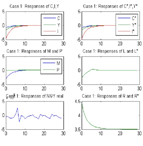
the usefulness of the model for the purpose of the next chapter, and also to explain in detail the behavior of the economies in the presence of shocks and for the two monetary policy regimes. The three subsections below analyze the behavior of the economies in the presence of negative shocks: first, a recession caused by a negative government consumption shock in economy H; second, a recession caused by a negative technological shock in economy H, andfinally a recession caused by a positive shock in monetary policy, i.e., an increase in the nominal interest rate.3
Variables in the figures presented below are real consumption (C), real investment
3In this section we use speci
fic parameter values for Czech Republic, that are calculated in Chapter 2,
18
(I), real output (Y), money (M), prices (P), labor (L), nominal interest rate (R), and net exports in percentage of GDP (NX
Y ). The superscript ∗ identifies foreign variables.
Impulse response functions represent deviations from the steady-state values, except in the cases of the nominal interest rates.
1.3.1
Government Consumption Shocks
Figure 1.1 shows impulse response functions for a negative government consumption shock in theCommon Monetary Policy regime. When a negative government consumption shock hits the domestic economy, output decreases initially in the first period and labor falls in the first six periods. In contrast, a decrease in government consumption makes private consumption increase. This effect results from the fact that consumers expect net taxes to decrease after a fall in government consumption, and therefore they increase present consumption.
Labor falls because consumption increases for the same level of work; this is caused by the anticipated increase in wealth (due to the expected fall in taxes), but most of all because firms have reduced production and therefore need fewer workers.
The movements of domestic and foreign consumption and investment are closely cor-related because they follow the same interest rate when making their decisions and also because the calibrated trade share between the country and the foreign economy (the Eu-rozone) is large; this leads to a close correlation between the movements of output and hence of the production factors.
Because consumption and investment rise, output also begins to increase after thefirst period, due to the rise in demand for the final good. Final good producers increase their demand for intermediate goods in order to satisfy the increasing demand for thefinal good. Prices of thefinal good fall, both in the domestic economy and in the foreign economy. Final goods price in the foreign economy decreases as a result of higher labor supply which makes the marginal utility of work decrease thus reducing marginal costs; hence, prices of intermediate goods that influence the price of the final goods also go down.
demand. The nominal interest rate decreases in thefirst period because output and prices have decreased in both the foreign and domestic economy. A lower interest rate in the first period and a higher consumption level push money demand up. When the interest rate starts to increase, money demand and consumption decrease.
Exports movements depend on consumption and investment related movements. Due to the existence of complete markets, the risk sharing effect prevails and exports decrease initially. The domestic economy is borrowing resources from the foreign economy, trigger-ing higher consumption in both economies.
20
Figure 1.1: Common Monetary Policy - Government Shock
In theAutonomous Monetary Policy regime, a negative shock in government
on foreign intermediate goods.
The nominal domestic interest rate falls in the first periods, because output has de-creased, although prices have increased. The drop in the interest rate does not happen for as many periods as in the previous regime, because of the increase in prices in the domestic economy. The movements of domestic and foreign consumption and investment are negatively correlated because the changes in their respective nominal interest rates are the opposite, with the domestic interest rate decreasing in the final periods and the foreign rate increasing.
22
1.3.2
Technological Shocks
The difference between Common Monetary Policy and Autonomous Monetary Policy re-garding technological shocks relies mainly in the behavior of net exports, as can be seen in Figures 1.3 and 1.4 below. In the first regime net exports increase, while falling in the second regime. In thefirst regimeHis selling goods toF, since output in the foreign econ-omy increases slightly, because the common nominal interest rate decreases in response to the negative domestic technological shock, increasing demand for both domestic and foreign intermediate goods.
When monetary policy is governed by the National Central Bank, the domestic nominal interest rate decreases by more when the negative domestic technological shock occurs and decreases domestic output, since it responds more to the conditions of the domestic economy. Domestic consumption and investment increase more in this regime and the domestic economy is borrowing resources from the foreign economy.
24
Figure 1.4: Autonomous Monetary Policy - Technological Shock
1.3.3
Monetary Policy Shocks
the domestic economy.
An increase in the nominal interest rate also makes mark-ups higher; as this increases monopoly power, it makes output decrease.
Figure 1.5: Common Monetary Policy - Monetary Shock
In theAutonomous Monetary Policyregime, which can be seen in Figure 1.6, a positive
26
decrease, these movements also lead to an increase in the balance of trade, because the domestic economy is lending resources to the foreign economy, since domestic investment decrease due to the increase in the nominal interest rate. Initially, output in the for-eign economy falls but investment initially increases. Labor decreases initially due to the decreasing domestic and foreign demand.
1.4
Discussion
In this chapter we build a two country dynamic stochastic general equilibrium model which allows for different monetary policy regimes. In one regime the domestic country belongs to the Eurozone, and the ECB policy rule responds to a weighted average of the economic conditions, mainly, of the inflation rate and output gap of the Eurozone members. The other monetary policy regime is one where the home country is autonomous of the Eurozone and decides on its monetary policy through its National Central Bank. The first monetary policy regime is a theoretical innovation in this type of models and a more realistic way to model the policy rule of the ECB.
This model with these two different monetary policy regimes is being used in the next chapter to quantify the economic cost of the loss of monetary policy flexibility. In order to assess the fitness of this model for the stated purpose, we analyzed impulse response functions of the model regarding government consumption, technological and monetary policy shocks, in the two different monetary policy regimes. The model behaves as expected regarding the analyzed shocks and it seems reasonable to use for the purpose of the next chapter.
28
1.5
Appendix A - First Order Conditions
1.5.1
Consumers
In each period t = 0,1, ..., consumers choose consumption, labor, real money balances, and bond holdings to maximize their utility:
E0
∞
X
t=0
βtU(ct, lt, Mt/Pt)
subject to the consumer budget constraints:
Ptct+Mt+Et+1QtBt+1
≤ PtWtlt+Mt−1+Tt+Qt−1Bt+Πt
The first order conditions for the consumer can be written as:
−U
l t
Uc t
=Wt
Utm Pt −
Utc Pt
+βEt+1
Ut+1c Pt+1
= 0
Qt−1=βEt−1
Uc t
Utc−1 Pt−1
Pt
where Uc
t, Utl and Utm are the derivatives of the variables of the utility function. We can
define the nominal interest rate, rN, from the lastfirst order condition:
1
1 +rN =βEt+1
Ut+1c Uc
t
Pt
Pt+1
The foreign consumer faces a similar problem to that of the domestic consumer, namely to maximize:
E0
∞
X
t=0
βtU(c∗t, l∗t, Mt∗/P∗t)
Pt∗c∗t+Mt∗+Et+1Q∗tBF
∗
t+1+Et+1QtBH
∗
t+1/et
≤ Pt∗Wt∗l∗t+M∗t−1+T∗t+Q∗t−1BFt∗+Qt−1BHt ∗/et+Π∗t
where BH∗ and BF∗are respectively, the foreign’s holdings of home and foreign country bonds. The first order conditions are similar to the ones for the domestic consumer, and the first order conditions with respect to bonds are:
Qt−1=βEt−1
Uc∗
t
Uc∗
t−1
Pt∗−1 Pt∗
et−1
et
Q∗t−1=βEt−1
Utc∗ Uc∗
t−1
Pt∗−1 Pt∗
If we equate the first order condition for the domestic bonds holdings for the foreign consumer and the first order condition for the domestic bonds holdings of the domestic consumer, we get:
Uc t
Utc−1 Pt−1
Pt
= U
c∗ t
Utc−∗1 Pt∗−1
Pt∗ et−1
et
With this expression and defining the real exchange rate as
qt=etPt∗/Pt
we get:
qt=ξUtc∗/Utc
by iterating back to 0, where ξ is the real exchange rate at time 0, times the ratio of the marginal utilities at time 0.
1.5.2
Final Goods Producers
30
maxP y−
1
Z
0
PiHyiHdi−
1
Z
0
PiFyiFdi
subject to
yt=
⎡ ⎢ ⎣a1
⎛ ⎝
1
Z
0
(yHi,t)θdi
⎞ ⎠
ρ θ
+a2
⎛ ⎝
1
Z
0
(yi,tF)θdi
⎞ ⎠ ρ θ⎤ ⎥ ⎦ 1/ρ
The first order conditions of the maximization problem for thefinal goods producers, with respect to yHi and yFi , respectively are:
yHi =
"
a1P y1−ρ¡R(yHi )θdi
¢ρ θ−1
PH i
# 1 1−θ
yiF =
"
a2P y1−ρ¡R(yFi )θdi
¢ρ θ−1
PF i
# 1 1−θ
raising the expression to the power θ, integrating acrossi, solving forR(yiH)θdi, and sub-stituting these expressions in the FOC stated above, we get the factor demand functions:
yHi,t=[a1Pt]
1 1−ρPH
t−1(1−ρρ)(θ−θ−1)
Pi,tH−11−1θ
yt
yFi,t=[a2Pt]
1 1−ρPF
t−1(1−ρρ)(θ−θ−1)
PF i,t−1
1 1−θ
yt
where PHt−1 is the average price of inputs and is equal to:
PHt−1=
⎛ ⎝
1
Z
0
Pi,tH−11−θ1 di
⎞ ⎠
θ−1
θ
and PFt−1 is equal to:
PFt−1=
⎛ ⎝
1
Z
0
Pi,tF−11−θ1 di
⎞ ⎠
θ−1
since all producers behave competitively, their economic profit is zero, and thefinal good price is given by:
Pt=
µ
a
1 1−ρ
1 P
H t−1
ρ ρ−1 +a
1 1−ρ
2 P
F t−1
ρ ρ−1
¶ ρ ρ−1
which is independent of period tshocks.
The problem for foreignfinal goods producers is equal and by solving it we get:
yi,tF∗=[a1Pt]
1 1−ρPF∗
t−1(1−ρρ)(θ−θ−1)
PF∗
i,t−1
1 1−θ
y∗t
yHi,t∗=[a2P
∗
t]
1 1−ρPH∗
t−1(1−ρρ)(θ−θ−1)
PH∗
i,t−1
1 1−θ
yt
Pt∗=
µ
a
1 1−ρ
1 P
F∗ t−1
ρ ρ−1 +a
1 1−ρ
2 P
H∗ t−1
ρ ρ−1
¶ ρ ρ−1
1.5.3
Intermediate Goods Producers
The domestic intermediate goods producers choose prices Pi,tH−1 and Pi,tH−∗1, production factors li,t,ki,t, andIi,tto maximize:
maxE0
∞
X
t=0
Qt[Pi,tH−1yi,tH+
+etPi,tH−∗1yH
∗
i,t −PtWtli,t−PtIi,t]
subject to the following production function:
yHi,t+yHi,t∗=F(ki,t−1, Atli,t)
and to the input demands derived from the final goods producers problem.
The law of motion for capital used in the production of the intermediate goodi is:
ki,t= (1−δ)ki,t−1+Ii,t−φ
µ
Ii,t
ki,t−1
32
and the constraints on prices are:
Pi,tH−1 =Pi,tH =...Pi,t+NH −1 PH
i,t+N =Pi,t+NH +1=...Pi,t+2NH −1
.
.
.
PH∗
i,t−1 =PH
∗
i,t =...PH
∗
i,t+N−1
PH∗
i,t+N =PH
∗
i,t+N+1=...PH
∗
i,t+2N−1
.
.
.
The derivatives of the Lagrangian with respect toPH
t−1and PH
∗
t−1 are:
X
τ=t
EτQτ
n
θPi,tH−1θ−11ΛH
τ −ζτPi,tH−1
2−θ θ−1ΛH
τ
o
= 0
X
τ=t
EτQτ
n
θePi,tH−∗1θ−11ΛH∗
τ −ζPH
∗
i,t−1
2−θ θ−1ΛH∗
τ
o
= 0
The derivative with respect toli,t is:
−PtWt+ζtFi,tl = 0
The derivative with respect toIi,tis:
−Pt+λt
∙
1−φ0
µ
Ii,t
ki,t−1
¶¸
= 0
and finally the derivative with respect to ki,t is:
−λt+Et+1Qt+1
½
ζt+1Fi,t+1k +λt+1
∙
1−δ−φ
µ
Ii,t+1
ki,t
+φ´
µ Ii,t+1 ki,t ¶ Ii,t+1 ki,t ¸¾ = 0
Pi,tH−1=
t+NP−1 τ=t
EτQτPτvi,τΛHτ
θt+NP−1
τ=t
EτQτΛHτ
Pi,tH−∗1=
t+NP−1 τ=t
EτQτPτvi,τΛHτ ∗
θt+NP−1
τ=t
EτQτeτΛHτ ∗
Uc t
1−φ0i,t =βEt+1U
c t+1
(
vi,t+1Fi,t+1k +
1 1−φ0i,t+1
∙
1−δ−φi,t+1+φ0i,t+1Ii,t+1 ki,t
¸)
where vi,t is the real unit cost which is equal to the wage rate divided by the marginal
product of labor, Wt/Fi,tl At and:
ΛHt = [a1Pt]
1 1−ρPH
t−1
ρ−θ
(1−ρ)(θ−1)y
t
ΛHt ∗= [a2Pt∗]
1 1−ρPH∗
t−1
ρ−θ
(1−ρ)(θ−1)y∗
Chapter 2
The Welfare Cost of the Loss of
Autonomy of Monetary Policy
2.1
Introduction
In this chapter we make use of the model built in the previous one, and use it to perform a welfare analysis for some countries, currently outside the Eurozone. The Czech Republic, Hungary, and Poland will have to join the European and Monetary Union (EMU) sometime in the future.1 On the other hand, Denmark, Sweden, and the UK have repeatedly refused to join the EMU. Surprisingly, there is very little work on the welfare consequences of the loss of monetary policy flexibility for these countries. Discussions are usually focused on the social and political consequences of the Euro, despite of the existence of a possible economic loss. This chapter fills this void by providing a quantitative evaluation of the economic costs of joining the EMU, specifically, by investigating the economic implications of the loss of monetary policyflexibility associated with EMU for each country at study.
We calibrate models specifically for each economy and use the model described in the previous chapter to perform simulations and calculate, through a welfare analysis, the economic costs of the loss of the monetary policy flexibility. By calculating a welfare analysis, the comparison of the two monetary policy regimes, i.e., to be outside or inside the Eurozone, aims, to assess whether or not consumers prefer a National Central Bank concerned with the effects of shocks in a given economy. We have never seen this done in 1These three transition countries were chosen because they are the biggest of the economies that joined
the European Union (EU) in May 2004.
the literature and for the purpose stated above.
Our focus is the loss of autonomy of monetary policy and its implications vis-a-vis
business cycle synchronization. Business cycle synchronization is an important decision factor for joining EMU. It is often argued that it is not a good decision to join the euro, if a country’s economic cycle is not synchronized with that of other remaining members as monetary policy may actually accentuate economic fluctuations. In the studies of Chamie, DeSerres, and Lalonde (1994) and Gros and Hefeker (2002) asymmetric shocks are discussed and also the level of asymmetry between regions. Both works compare the EU with the USA. Results show that the USA presents a higher level of symmetry between regions than the EU. This supports the fact that some European countries are going to suffer more than others from joining the Euro. Also, in face of shocks, European economies do not seem to converge or be symmetric in their responses, in fact they diverge.
Related literature for this topic and for transition countries is very recent. For the transition countries at study in this paper, Holtemöller (2005) calculated for the Czech Republic, Hungary, and Poland an optimum currency area index (OCA) to measure the economic consequences of joining the EMU, and uses a Taylor Rule similar to the one we use for the European Central Bank, but in a different economic framework. The author compares national monetary policy with monetary union in a two country new-keynesian model, but does not apply a general equilibrium framework. The OCA index measures the relative loss in terms of output gap and inflation variability in the two regimes stated above. He concludes that both the Czech Republic and Hungary can reduce the volatility of inflation and of the output gap if they join the monetary union. Results for Poland are inconclusive.
Fidrmuc and Korhonen (2003) have done calculations of correlations of supply and demand shocks between the accession countries and the Eurozone. They conclude that EMU accession would be easy for Hungary, and have mixed results for Poland and Czech Republic. They also present some review of literature of business cycle synchronization between Central Europe and Eastern Countries (CEECs) and the EMU.
36
the EMU increases the volatility of output and inflation and that loosing the ability to stabilize the domestic economy is less costly if supply shocks are small. They estimate that the UK stabilization cost for joining the EMU is equivalent to a permanent reduction in GDP of between 0.6% and 2%.
In the next section we present some calculations regarding the proportion of the busi-ness cycle explained by idiosyncratic factors. We show that for the developed countries at study, the specific component of the cycle is very high, but has been declining. On the other hand, Stock and Watson (2005) show that UK business cycle is less synchro-nized with the European business cycle and more with the North-American one, over the 1984-2002 period. They also concluded that the percentage of the business cycle that it is explained by country specific factors is increasing, contrary to other related literature, that points to the opposite result. This is also one of the five economic tests that the British Government analyzes from time to time in order to evaluate the benefits and costs of joining the EMU. Fidrmuc and Korhonen (2003) and Angeloni and Dedola (1999) are also relevant references for UK, Sweden, and Denmark for this topic.
In section 2.2 we present empirical evidence regarding synchronization and conver-gence for the economies at study. In section 2.3 we show the calibration procedure and reference values for the six countries. Section 2.4 discusses the methodology and sections 2.5 and 2.6 analyze results for the welfare cost of the loss of monetary policy flexibility and sensitivity analysis for transition countries. Sections 2.7 and 2.8 do the same for the developed countries and section 2.9 concludes and presents a discussion of the results, some limitations of this work, and suggestions for future research. Sections 2.10 to 2.13 present some additional information about data, calibration, business cycles statistics, and welfare results.
2.2
Empirical Evidence
opt-out clause.
Hungary plans to join the Euro in 2010 and join the European Exchange Rate Mecha-nism II (ERM II) as soon as convergence criteria are met. Its currency is currently pegged to the Euro with a wide band of 15%. Poland plans to join the Euro in 2011; despite this goal, it has no target date for joining ERM II and its currency is currently floating. The Czech Republic has not yet set a date for joining the Euro but aims to join the ERM II when convergence criteria are achieved. Its currency is on a managed float.
The economic conditions of these countries do not differ much from those of Portugal and Greece, the poorest of the European Union economies, at the time of their accession, as we can see in Table 2.1. GDP per capita in these economies resembles the levels,
at the time of accession, for Portugal and Greece. These countries are also small open economies like Portugal and Greece, but much more open to trade. This makes them specially vulnerable to shocks and highly dependent on foreign trade partners.2
Table 2.1 - Comparison of GDPper capita and Degree of Openness in the Accession Year Countries (Year of Accession) GDPper capita in PPP (EU-15=100) Degree of Openness
Greece (1981) 63% 27.2%
Portugal (1986) 53% 28.7%
Czech Republic (2004) 65% 71.3%
Hungary (2004) 56% 65.1%
Poland (2004) 45% 38.5%
Data Source: NewCronos
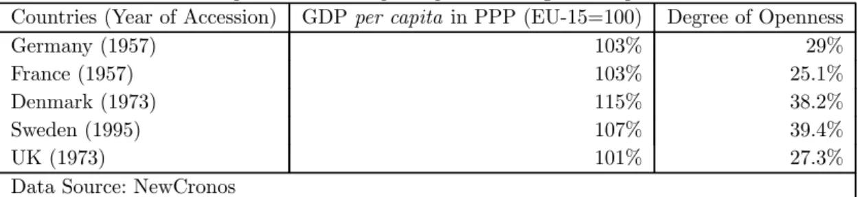
Unlike the referred three countries, Denmark, Sweden, and the United Kingdom have repeatedly refuse to join the Euro. These are developed economies, with GDP per capita
comparable to, or even higher than Germany and France, values that are shown in Table 2.2. Their situation is opposite of the one of the transition countries, by the time of the introduction of the Euro, in 1999. Denmark and Sweden are more open than Germany and France, but the UK has roughly the same degree of openness. These countries are however, relatively less dependent on foreign trade than the transition countries at study. 2Degree of Openness is calculated as [(exports+imports)/2]/GDP*100. The variables are in nominal
38
Table 2.2 - Comparison of GDPper capita and Degree of Openness in 1999
Countries (Year of Accession) GDPper capita in PPP (EU-15=100) Degree of Openness
Germany (1957) 103% 29%
France (1957) 103% 25.1%
Denmark (1973) 115% 38.2%
Sweden (1995) 107% 39.4%
UK (1973) 101% 27.3%
Data Source: NewCronos
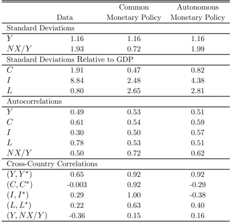
Business cycle synchronization is also an important decision factor to join the EMU. If business cycles are not synchronized, the impact of a common monetary policy is different for each country and may hurt the economy of the country. The ECB considers only the average economic condition of the Eurozone when setting monetary policy. Table 2.3 shows results for the cross-country correlations between the countries at study and the Eurozone.3 We can see that Poland has a significative positive correlation with the Eurozone for output (Y) and investment (I) and a slightly lower positive correlation with labor (L), and consumption (C). Hungary has a strong positive correlation with the Eurozone output and a lower positive correlation for investment and labor. Consumption does not appear to be correlated. Synchronization does not exist between the Czech Republic and the Eurozone, with all the correlations for the variables being negative. Data for obtaining the statistics for these countries is very time limited, so results must be read with care.
For developed countries output, investment, and labor correlations are positive for all countries. Consumption correlation of Denmark and of the UK is negative, but of Sweden is significantly positive. Correlations between the UK and the Eurozone are the weakest ones and Sweden has the strongest degree of comovement with the Eurozone.
Table 2.3 - Cross-Country Correlations between the Countries and the EMU
CZ HU PL DK SE UK
(Y, Y∗) -0.15 0.65 0.52 0.53 0.67 0.19
(C, C∗) -0.49 -0.003 0.23 -0.03 0.72 -0.02
(I, I∗) -0.18 0.29 0.72 0.38 0.72 0.22
(L, L∗) -0.36 0.22 0.06 0.51 0.70 0.26
3See Appendix C for details on empirical data and methodological issues. The superscript
Also important is the proportion of the economic cycle of each country that is explained by an idiosyncratic component vis-a-vis a common component with the Eurozone.4 If the
idiosyncratic component is very high that could be a problem for EMU accession, because the lower the correlation between the economic cycle of a country and the Eurozone, the bigger could be the welfare loss of giving up monetary policy. For the sake of comparison we also present results regarding the common component with the USA. Results for the countries at study are presented in Tables 2.4 and 2.5.
Table 2.4 - % of the Variability of the Specific Component in the Total Variability of the Cycle
1992-2004 Eurozone USA Czech Republic 0.38 0.39
Hungary 0.13 0.16
Poland 0.15 0.21
Table 2.5 - % of the Variability of the Specific Component in the Total Variability of the Cycle
1960-1978 1979-2004 1960-2004 Eurozone USA Eurozone USA Eurozone USA
Denmark 0.53 0.91 0.48 0.60 0.56 0.78
Sweden 0.60 0.71 0.30 0.47 0.58 0.64
United Kingdom 0.73 0.80 0.40 0.42 0.59 0.58
As we can see, the weight of the specific component is small in the three transition countries, but specially small in Hungary and Poland. The proportion of the specific component is higher when we calculate for the USA, meaning that the proportion of the economic cycle explained by the Eurozone economic cycle is higher.
For developed countries, data availability allows us to divide the period between 1960 until 2004 in sub-periods. We choose to divide the data in the year 1979 because it is the starting year of the European Monetary System. The weight of the specific component has been declining over time, however the specific component in these countries is much bigger that the one of the transition countries. Denmark, Sweden, and the UK are bigger economies and much less open to trade, hence less affected by comovements of other countries. The specific component of business cycle of the UK is more or less the same
40
regardless whether we use the Eurozone or the USA, reflecting the strong relation between the UK and the USA, despite the accession to the European Union.
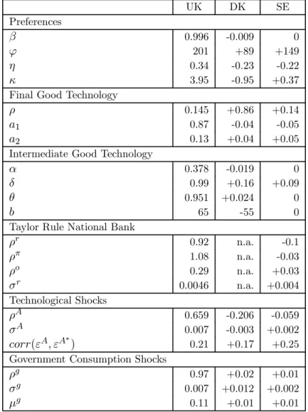
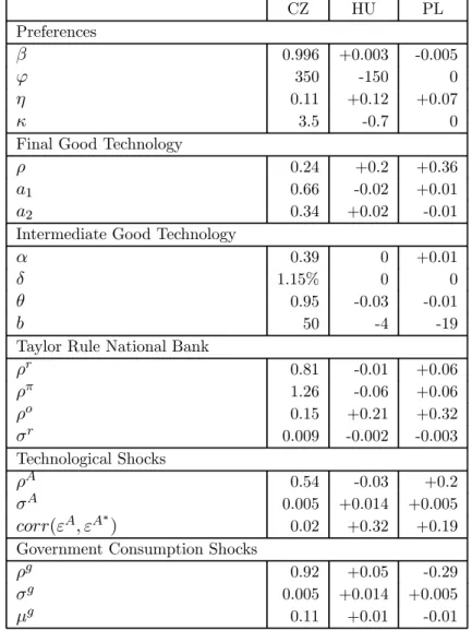
2.3
Calibration
The calibration of the model developed in the previous chapter is made in order to re-produce the long term properties of the economies at study. Parameter values for these countries are presented in Appendix B. We follow the calibration procedure of Cooley (1995).
2.3.1
Preferences
The functional form of the utility function is:
U
µ
c, L,M P
=
⎡ ⎣c(1−κ)
(1−κ) +
w(MP)
η−1
η
η−1
η
+ϕ(1−1l)−(1γ−γ)
⎤ ⎦
1−σ
1−σ (2.1)
whose arguments are real consumption (c), labor (l) and a real money aggregate (M/P). The discount factor β is equal to(1+r1LT), where rLT is the real long term interest rate for government bond yields. The value for σ is 0.0001 for all countries at study and
κ is the relative risk aversion coefficient (or the inverse of the elasticity of intertemporal substitution). The value for this parameter found in the literature, can vary between 1 and 20. Because this parameter is one of the most difficult values to estimate empirically, we perform a sensitivity analysis to the value of this parameter. In order to have a balanced growth we imposeγ=σ.5 The value forϕ, the weight on leisure, is calculated in order to match the time that families dedicate to work to empirical data.
5In the market sector suppose that technology for each intermediate good producer is given by
F(kt, Atlt), where At grows at a constant rateA. In the nonmarket sector suppose that technological
progress increases the productivity of time destined to nonmarket activities, so that an input of (1−lt)
units of time out of the market, produces At(1−lt)units of leisure services. With these kind of
prefer-ences, ifctandmt grow at aAtrate and ifltis constant, then−UUctlt =k(1+A)
(1−γ)t
(1+A)−σt wherekis a constant.
Parameters concerning money demand are estimated according to the first order con-dition for a nominal bond, which costs one euro att and pays(1 +rN) euros in t+ 1:
logMt
Pt
=−ηlog w
1−w+ logct−ηlog
µ
rN
1 +rN
(2.2)
we estimated a regression with quarterly data, where M1 is used for money, the GDP
deflator forP, private consumption at constant prices forc,and the three month interest rate of the money market for rN, whererN is the nominal interest rate. In the estimation
we obtained the value for η, the interest elasticity of real money demand. The value for
w is residual and we set the value equal to 0.0076 for all countries.
2.3.2
Technology for the Final Goods Producers
The elasticity of substitution between home and foreign goods was defined as (1−1ρ). Some studies, like the one by Whalley (1985), found this elasticity to be in a range between 1 and 2, being lower for Japan and Europe than for the USA. The value found for this elasticity is calculated by using the expression of thefirst order condition for the demand functions of the input intermediate goods:
logIM P
D =b0+b1log P D
P IM P+b2logY (2.3) whereIM P are imports at constant prices,Dis national production subtracted of exports at constant prices, P IM P is the imports deflator, P D is the deflator for D, and Y is national income at constant prices.
Shares for the model are calculated assuming that there are only two countries in the world, each one of the countries and the Eurozone. yh and yf represent the share of imports from the Eurozone in percentage of GDP and the share of national production in percentage of GDP, respectively. To calculate a1 and a2, representing respectively the
weights of domestic and imported goods, in their steady state values, the following relation is established: yh/yf = [a1/a2]