Batalin-Fradkin-Vilkovisky quantization of the generalized scalar electrodynamics

Batalin-Fradkin-Vilkovisky quantization of the generalized scalar electrodynamics

Instituto de Fı´sica Teo´rica (IFT), UNESP-Sa˜o Paulo State University, Rua Dr. Bento Teobaldo Ferraz 271-Bloco II, Barra Funda, Sa˜o Paulo, CEP 01140-070 Sa˜o Paulo, Brazil

(Received 17 December 2012; published 10 September 2013)

This work comprises a study upon the quantization and the renormalizability of the generalized electrodynamics of spinless charged particles (mesons), namely, the generalized scalar electrodynamics (GSQED4). The theory is quantized in the covariant framework of the Batalin-Fradkin-Vilkovisky

method. Thereafter, the complete Green’s functions are obtained through functional methods and a proper discussion on the theory’s renormalizability is also given. Next, we present the computation and further discussion on the radiative correction atorder; and, as it turns out, an unexpectedmP-dependent divergence on the mesonic sector of the theory is found. Furthermore, in order to show the effectiveness of the renormalization procedure on the present theory, we also give a diagrammatic discussion on the photon self-energy at2 _{order, where we observe contributions from the meson self-energy function.}

Afterwards, we present the expressions of the counterterms and effective coupling of the theory, obtaining from the latter an energy range where the theory is defined bym2_k2_{< m}2

P. We also shown in our final discussion that the new divergence is absorbed suitably by the mass countertermZ0, showing therefore

that the gauge Ward-Fradkin-Takahashi identities are satisfied still.

DOI:10.1103/PhysRevD.88.065013 PACS numbers: 11.10. z, 11.10.Gh

I. INTRODUCTION

Higher-order derivative (HD) Lagrangians [1] are a fairly interesting branch of the ongoing effective theories [2] in these thrilling times of high-energy physics we are living in. It is known that HD theories have, as a field theory, better renormalization properties than the conven-tional ones. These properties have shown to be quite ap-pealing in the attempts to quantize gravity, where the Einstein action is supplied by terms containing higher powers of curvature leading to a renormalizable [3] and asymptotically free theory [4]. Also, nowadays a new impetus in exploring appealing quantum theories of gravity has arisen, for instance the fðRÞ gravity [5], which is a strong candidate for explaining the accelerating universe. Higher derivative theories were proposed initially as an attempt to enhance and render a better ultraviolet behavior of physically relevant models [6]. Once the effective theory is rendered ultraviolet (UV) finite, we may consider it an extension of the class of potentially interesting and con-sistent models because its UV dynamics is now well de-fined. However, it was soon recognized that they possess a Hamiltonian that is not bounded from below [7] and that the process of adding such terms leads to the existence of negative norm states (or ghosts states) on the quantum theory—induces an indefinite metric in the space of states—jeopardizing therefore the unitarity of the theory [8]. Despite the fact that many efforts have been made to overcome these ghost states, none of them has been able to give a general method to properly cope with this major

problem [4,9,10]. From the point of view of effective field theories, a field theory violating unitarity might still be sensitive at a low energy as long as the ghosts states are unstable so that they do not appear as asymptotic states.

As pointed out in several works [11–13] along the years, it is long clear that Maxwell’s theory is not the only one to describe the electromagnetic field. One of the most suc-cessful generalizations is generalized electrodynamics [11]. Actually, Podolsky’s theory is the only one linear, Lorentz, and Uð1Þ invariant generalization of Maxwell’s theory [13]. Another interesting feature inherent to Podolsky’s theory is the existence of a generalized gauge condition also, namely, the generalized Lorenz condition: ½AŠ ¼ ð1þm 2

P hÞ@A [14]; considered an important issue, it is only through the choice of the correct gauge condition that we can completely fix the gauge degrees of freedom of a given gauge theory [14]. The authors with collaborators have also been studying Podolsky’s theory at finite temperature [15,16] and some interesting results were obtained, such as implications on Podolsky’s free parameterm_P.

In a series of previous works [17,18], we have presented the quantization and the renormalization of the generalized quantum electrodynamics (GQED₄). The outcome in these works was encouraging as we observed that the theory’s ultraviolet divergence was partially canceled at order. The electron self-energy and vertex part are both UV finite at order only whether the generalized Lorenz condition is considered. Another interesting point considered in the previous paper was the use of the experimental data of an electron’s anomalous magnetic moment to bound possible values of the free parameterm_P; from such calculations we found a consistent value of m_P3;75951010 _eV. *_{[email protected]}

In our opinion, the success of the theory of generalized quantum electrodynamics warrants a similar investigation for other elementary particles. A first step towards this direction is considered in the present paper, which is the study of the interaction of charged spinless mesons with the Podolsky electromagnetic field. We shall denote this theory as the GSQED4. Although a proper discussion on scalar electro-dynamics features is a rare subject to find in the literature [19], there is an outstanding study of scalar electrodynamics pre-sented in rich details and proofs in Ref. [20]. On theoretical grounds,GSQED4is an attractive theory, once its interaction Lagrangian contains a richer structure than its fermionic counterpart. The use of spinless fields is fairly motivated in order to elucidate complicated properties of a given theory, once it simplifies calculations in a theory due to its spinless character and other nuances. Examples of that can be found in investigations concerning QCD properties [21], in which it is believed that perturbative results (analytical results) can pro-vide a natural guide to possible nonperturbative structures.

Therefore, in this paper, we shall present a detailed study of the generalized scalar quantum electrodynamics from a functional integral point of view. The main focus of the present discussion will be the analysis of the divergent behavior of GSQED4. The structure of the paper is as follows. In Sec. II, we present a study of the canonical structure of the theory by following the Ostrogradski method to approach higher-derivative theories, and subsequently we construct the theory’s transition amplitude through the Batalin-Fradkin-Vilkovisky (BFV) procedure [22]. Next, in Sec. III, we introduce the generating functional and, thereafter, we compute the fundamental Greens functions. Through this functional, we also derive the generalized Ward-Fradkin-Takahashi (WFT) identities in Sec. IV. In Sec.V, we apply to theGSQED₄the on-shell renormaliza-tion prescriprenormaliza-tion and also discuss the appropriated renormal-ization conditions. In Sec. VI, we evaluate the radiative corrections of the theory at the -order approximation; discussing deeply the details of the divergent structure of the resulting expressions. We also present a discussion on the divergent behavior of the photon self-energy function at 2 order. Next, in Sec.VII, we present the expressions for the counterterms and for the effective coupling of the theory as well. Our remarks and prospects are placed in Sec.VIII. The Minkowski spacetime is concerned in the whole work, with the metric signature (þ; ; ; ).

II. CONSTRAINT ANALYSIS AND TRANSITION AMPLITUDE

It is well known that effective theories may or may not be unitary. The unitarity is lost when a particle can lower its energy by emitting other particles that have been eliminated in deriving the effective theory. Actually there are sufficient reasons to dismiss any quantum theory, such as Einstein gravity, that had the presence of HD quantum corrections and ghosts states. Motivated by the search of possible

fundamental theories, one may naturally expect the com-plete suppression of nonphysical, nonunitary processes. Nevertheless, in this paper we will assume that, although we are not giving here a formal proof upon the details of physical space for Podolsky’s theory, an analysis could be performed, for example through the generalized Kubo-Martin-Schwinger boundary conditions [23], or by the Becchi-Rouet-Stora-Tyutin (BRST) symmetry and quartet mechanism [24], or even by the scheme proposed by Hawking and Hertog [9], leading therefore to a well-defined theory of the generalized electrodynamics. In the following, we shall give a brief derivation on the constraint structure of GSQED₄ in order to construct the transition amplitude through the BFV method. Therefore, we have that the Lagrangian density describing the generalized scalar electrodynamics is given by

L¼ ðD’ÞyD’ m2’y’ 1 4FF

þ 1 2m2

P

@F_@F

; (1)

where F¼@A @A is the usual electromagnetic field-strength tensor, and D’¼@’ igA’ is the covariant derivative. The interaction terms of the model Eq. (1) can be written explicitly as

L_¼@’y_{@’ m}2_’y_’þig’y$_@’A

þg2_A

’yA’ 1 4FF

_þ 1

2m2 P

@F_@F :

(2)

Furthermore, the Lagrangian density (1) is invariant, at the classical level, under the local transformations:

’ðxÞ !eigðxÞ_{’ðxÞ; A}

!Aþ@ðxÞ: (3) The Euler-Lagrange equations following from Hamilton’s principle [12] are

ðhþm2_{Þ’ igð2@}

’Aþ’@AÞ g2AA’

¼0; (4)

and

ð1þm 2

P hÞ@F¼j; (5)

where j_¼ig’y$_@’þ2g2_’y_{A’ is the scalar} four-current.

In order to study the constraint structure of the present model, we must first compute the canonical momenta of the field variables. Thus, the canonical momenta associated with the scalar fieldsð’; ’y_Þare

p¼ @L

@ð@₀’y_Þ¼@0’ ig’A0;

p¼ @L

@ð@₀’Þ¼@0’

y_þig’y_A

0;

whereas the canonical momenta for gauge fields are ob-tained from the Ostrogradski method to higher-order theo-ries [1]. This method consists of defining the dynamics of the system in a spanned phase space characterized by the independent variables ðA; _{Þ and ð}

@0A; Þ. Therefore, it follows that the generalized momenta asso-ciated withðA; Þ[14,25] are given by

_¼ @L

@ð@0 Þ

¼ 1 m2

P

ð0_@

F0 @FÞ; (7)

_¼ @L @ð Þ 2@k

_@L

@ð@_k Þ

@₀

_@L

@ð@₀ Þ

¼F0 1 m2_Pð

k_@

k@F0 @0@FÞ: (8)

From Eqs. (7) and (8), and according to the linear independence of the constraints [25], one obtains the following set of first-class constraints:

1 ¼ 0 0; 2 ¼0 @k k0;

3 ¼@k

k igðp’ p’ yÞ 0;

(9)

which comes strictly from the gauge sector, and no second-class constraint is obtained. Here represents the fact that (9) are weak equations, according to Dirac’s procedure [25].

As mentioned earlier, we will follow here the covariant framework of the BFV method [22] to construct the tran-sition amplitude for the model:

Z¼Z DAkDkD lD lD’yD’DpDpDDbD cDcD PDP

exp

iZ d4_x½

kA_kþ k_kþ ð@0’yÞpþ’p_ þc_Pþð@0cÞPþb_ HCŠ þi

Z

dw0f ; QBRSTg

; (10)

with the quantities being defined byðc;PÞandðc; P Þ, the ghost fields and its conjugated momenta, as ð; bÞ is a Lagrange multiplier and its momentum, all satisfying the following Berezin brackets:

fcðzÞ; PðwÞg_B¼ðz; wÞ; fðzÞ; bðwÞg_B¼ðz; wÞ;

fPðzÞ; cðwÞg_B¼ ðz; wÞ: (11)

The canonical HamiltonianH_C is given by

H_C ¼0 0þj jþ m2

P

2 l

l_þ l@l 0

þ _l@_kFlk_{þpp þigðp’ ’}y_pÞA

0

@_k’y_@k_’þm2_’y_{’ ig’}y$_@k_’A k

g2_A

k’yAk’ 1

2ð j @jA0Þ 2_þ1

4FkjF kj

1 2m2

P

ð@j

j @j@jA0Þ2: (12)

Another quantity that presents in (10) is the BRST charge Q, which has here the following form:

Q_BRST¼Z d3_z½c½@

kk igðp’ p’ yފ iPbŠ: (13)

The quantity remaining to be defined here is the gauge-fixing function . Actually, one of the remarkable features of the BFV method is that the quantization procedure is independent of the choice of this function [22]. However, we will work here at the generalized radiation gauge condition

4 ¼A0 0; 5¼ 0 0;

6 ¼ ð1þm 2

P hÞ@kAk0;

(14)

which hence allows us to write

¼Z d3_wi

2bcþicð1þm 2

P hÞ@kAk ð1þmP2hÞ 1P

: (15)

Therefore, by computing f ; QBRSTg and substituting its resulting expression into (10), and then carrying out the momenta and field variables integral, one finds the following expression for the transition amplitude:

Z¼Z DAD’yD’DcDc exp

iZ d4x

ðD’ÞyD’ m2’y’ 1 4FF

_þ 1

2m2 P

@F@F

1

2½ð1þm 2

P hÞ@AŠ2þi@cð1þmP2hÞ@c

Hence, from the BFV formalism we have obtained directly the desirable covariant expression for the transition ampli-tude. Furthermore, we see that the ghosts fields are de-coupled from the gauge fields, and so, their contribution can be absorbed into a normalization constant.

III. SCHWINGER-DYSON-FRADKIN EQUATIONS

In the present section, we continue the formal develop-ment of theGSQED4, by deriving now coupled relations between the fundamental Green’s functions, which are known as the Schwinger-Dyson-Fradkin equations (SDFE) [26]. We will consider the theory’s fundamental

Green’s functions: the gauge field propagator D, the me-son field propagator S and the two vertex functions, the three-point function , and the four-point function. For the derivation of these quantities we will make use of the functional methods, which provide a rather natural way to obtain such functions. In this context, we need to define the generating functional:

Z½;; J Š ¼Z Dð’; ’y_{; A}

Þexp½iAŠ; (17)

with the actionAgiven by

A_¼Z_d4_xðD

’ÞyD’ m2’y’ 1 4FF

_þ 1

2m2 P

@_F

@F

1

2½ð1þm 2

P hÞ@AŠ2þ’ þ’yþJA

;

¼A_effþZ d4_{x½’ þ’}y_þJ

AŠ: (18)

The sources,, and Jare related with the fields’y_,’,

andA, respectively.

A. SDFE for the photon propagator

We will derive here the complete expression of the photon propagator. In order to obtain its SDFE equation, we need to solve

_A

eff AðxÞ

i; i;iJ

þJ_{ðxÞZ½;; J}

Š ¼0; (19)

which, when used (18) for the actionA_eff, can be rewritten as

iJ_ðxÞZ¼D Z

J_ðxÞþglim_z!x½@ x @zŠ

2_Z ðzÞðxÞ

2g2 3Z

JðxÞðxÞðxÞ; (20)

where we have already defined the differential operatorD as the following:

D_¼

hT_þ1 ð1þm

2

P hÞhL

ð1þm_P2hÞ;

(21)

with the following set of differential projectors: T_þ L_¼;L¼@_@

h .

It is interesting for our purposes to introduce new useful quantities related to the generating functional Z. Hereby, we first introduce the generating functional for the con-nected Green’s functionsW, which is defined by the rela-tionW ¼ ilnZ. It proves convenient to introduce also the generating functional for the 1PI Green’s functions, which is related toW through a Legendre transformation:

½’; ’y_{; A}

Š ¼W½; ; J Š

Z

d4_{z½’ þ’ þJ} AŠ:

(22)

From the above definitions, one can obtain identities relating the connected and 1PI two-point functions. For instance, it follows that for the meson field

Z

d4_x 2 ’ðyÞ’ðxÞ

2_W

ðxÞðwÞ¼ ðw; yÞ: (23)

We also have the gauge field functionals satisfying a similar relation as the above. Actually, these identities, such as (23), are an important key for the formal develop-ment through functional methods and they will be used quite often throughout the work. Anyhow, writing (20) now in terms of W and then differentiating the resulting expression with respect toJ_{ðyÞit follows that}

ðx; yÞ ¼Dx

2W

J_ðyÞJðxÞþglim_z!x½@ x @zŠ

3W J_{ðyÞðzÞðxÞ}

2g2_lim z!x

4_W

JðxÞJ_{ðyÞðzÞðxÞ}þi

2_W ðzÞðxÞ

2_W JðxÞJðyÞ

: (24)

ðx; zÞ ¼ glim h!x½@

x

@hŠð1Þðx; h;zÞ þ2g2lim

h!x½ð2Þðx; h;zÞ iðx; zÞ

Sðx; hފ; (25)

with the quantitiesð1Þ andð2Þ defined by (A1) and (A2),1 respectively, and also, by identifying Dðw; xÞ, Eq. (A12), as the photon complete propagator, one obtains from (24) the complete expression for the propagator of the photon field in the Fourier space:

iD¼

kk

k2 k2_{½ðkÞ þ ð1 m} 2

P k2ފ

þ

k2_{ð1 m} 2 P k2Þ2

kk k2 :

(26)

The functionalis known as the polarization tensor, or photon self-energy function, and it is related to the scalar polarizationthrough the structure

_{ðkÞ ¼ ð k}2_{þkkÞðkÞ: (27)}

Differently from the generalized quantum electrodynamics [17], the scalar version possesses new interaction terms and, consequently, a richer and rather interesting structure on its radiative functions (25). We will present the evalu-ation of the radiative correction functions at the lowest order, and respective discussion on them, in the Sec.VI.

Furthermore, the photon propagator at the lowest order in perturbation theory can be conveniently written as

iD¼

ð1 Þkk k2

₁

k2

kk

k2 _m2 P

1 k2 _m2

P

þ ð1 2Þ kk k2_ðk2 _m2

PÞ

: (28)

The above expression shows explicitly the contribution from the ghost states; and as we stated earlier, we will assume here that an analysis could be performed on that leading, hence, to a well-defined theory to the generalized electrodynamics. Also we are motivated to retain some attention to the present theory, once its fermionic counter-part showed to be a rich theory, possessing a UV finite

behavior (at the light of effective theories) and interesting renormalized behavior.

Actually, the major feature of the structure of the photon free propagator (28) is observed when it is applied to radiative correction calculation. As it was shown in a previous paper [17], the contribution from the m_P-dependent terms act as enhancing the UV behavior and eliminating the UV divergences of some sectors of GQED₄. However, as it was pointed out, this remarkable result is only attainable in the presence of a suitable gauge condition, the generalized Lorenz condition [8]. This point will be further discussed in the Sec.VI.

B. SDFE for the meson field propagator

In this subsection we will continue the derivation of the theory’s SDFE, obtaining now an integral expression for the complete meson propagator S. We will follow the guidelines presented previously on the derivation of the photon propagator. Thereafter, we must first solve the following equation:

_A

eff ’ðxÞ

i; i;iJ

þðxÞ

Z_{½;; J Š ¼0: (29)}

After a careful evaluation of the functional derivative of

A_eff one can find the expression

ðhþm2_Þ Z

ðxÞþglimz!x½2@ x þ@zŠ

2_Z J_ðzÞðxÞ

þg2

3_Z ðxÞJðxÞJðxÞ

¼iðxÞZ ₍₃₀₎

Now, writing the above Eq. (30), in terms of the generating functionalWand then differentiating the resulting expres-sion with respect to the sourceðyÞ, one obtains

ðx; yÞ ¼ ðhþm2_Þ 2W

ðyÞðxÞþglimz!x½2@ y þ@zŠ

3_W J_{ðzÞðyÞðxÞ}

þg2 lim

z!x

4_W

JðxÞJðzÞðyÞðxÞþi

2_W ðyÞðxÞ

2_W JðxÞJðzÞ

: (31)

Next, we define the meson self-energy function through

ðz; yÞ ¼ glim h!x½2@

y þ@zŠð3Þðz; y; hÞ g2lim_h!x½ð4Þðz; y; h; xÞ iðy; zÞDðh; xފ; (32)

with the quantitiesð3Þandð4Þdefined by Eqs. (A3) and (A4), respectively. Hence, by taking the limit of null sources, having (A13) as the definition of the scalar

propagator, one then finds the following expression to the complete scalar propagator:

SðpÞ ¼ i

p2 _m2 _ðpÞ: (33)

It is easily seen from (33) that the free expression forS

does not differ from the one obtained on the usual theory. However, the self-energy function (32), different from the photon function Eq. (25), is sensitive to the effects of the Podolskym_P-dependent terms of (28) already at first order on perturbation theory.

We also have that the fairly investigated phenomenon in the scalar theory, the scattering light by light, at lowest order, does not change from the usual theory results once the expressions forSand three-point vertex (as we will show next) are not changed at the tree level [20].

C. SDFE for the vertex’y’A

The starting point for the derivation of the vertex func-tion [defined in (A14)] is Eq. (30), and its resulting

expression also follows from the guideline presented previously. Anyhow, we should write (30) first in terms of the generating functionalW, and then after differentiat-ing it with respect to the source ðyÞ, we finally take the derivative of the resulting expression with respect to the fieldAðzÞ. However, although the calculation is straight-forward, but quite long, it adds nothing new or relevant for the theory discussion. Hence, we present only its final expression in the following form:

_{ðx; y;zÞ ¼ ilim} h!x½2@

y þ@hŠðh; zÞðy; xÞ þðx; y;zÞ;

(34)

where we have also defined a new quantity, the vertex part by

ðx; y;zÞ ¼gð6Þðx; y; zÞ þlim h!x½2@

y þ@_hŠð5Þðx; y; h; zÞ 2ig2ðz; xÞ

Z

d4_sd4_{fDðf; xÞ}

ðs; y;fÞSðx; sÞ;

(35)

with the quantities ð5Þ and ð6Þ defined by the Eqs. (A5) and (A6), respectively.

As is well known, the SDFE do not only depend on the fundamental Green’s functions of a given theory, but they do depend on higher-order functionals, which also satisfy their own SDFE. For instance, the three-point vertex func-tion depends on the four-point one, which in turn depends on the five-point one, and so on. However, once we are only interested in perturbative calculation, the situation here is not that complex, since we have only four fundamental Green’s functions. Also, it is known that all the higher vertices can be defined in terms of the fundamental quan-tities via Feynman diagrams [27].

D. SDFE for the vertex’yA’A

In the same way as for the three-point vertex func-tion , the starting point to derive [defined in (A15)] is to take suitably appropriated functional deriva-tives of Eq. (30). Thus, following the same guideline, we write it in terms of the generating functional W, then differentiate it with respect to the source ðyÞ, and we finally take the derivative of the resulting expression with respect to the fieldsAðzÞandAðsÞ. However, the formal development and the evaluation of each term is even longer than as for . Therefore, we present only its final expression casted as

ðx; y;z; sÞ ¼2ðs; xÞðz; xÞðx; yÞ þ ðx; y;z; sÞ; (36)

with the vertex part defined as the following:

ðx; y;z; sÞ ¼lim

h!xð9Þðx; y; z; s; hÞ þ ð10Þðx; y; z; sÞ iðx; yÞð11Þðz; s; yÞ þð7Þ

ðx; y; zÞðs; xÞ

þð8Þðx; s; yÞðz; xÞ; (37)

where the quantities ð7Þ ð11Þ are defined by Eqs. (A7)–(A11), respectively.

The conclusions presented previously for also hold to the four-point vertex function.

IV. WARD-FRADKIN-TAKAHASHI IDENTITIES

The existence of a local gauge symmetry in a field theory generates constraint relations between the theory’s Green’s functions. These relations are known as the Ward-Fradkin-Takahashi identities. These identities, in terms of Green’s functions, protect the

equivalence on different gauge conditions. Also, as we shall see in Sec. V, these identities are also strictly related with the renormalizability of a theory. Hereby, we start the derivation of these identities from the following identity:

Z_{½;; J Š} ðxÞ

¼0

¼0: (38)

Thereafter, we find that the generating functional

ih gð1þm

2 P hÞ2@

JðxÞ

þ ðxÞ

ðxÞ

1 g@J

_{Z¼0: (39)}

Next, rewriting (39) as an equation for the generating functionalW½;; J Šit follows that

h

gð1þm 2 P hÞ2@

W JðxÞ

þi W ðxÞ i

W ðxÞ

1 g@J

_{¼0: (40)}

Finally, one can obtain the desired quantum equation of motion for the theory by writing (40) as an expression for the 1PI-generating functional ð’; ’y_{; A}

Þ through the relation (22). Hence, one gets

h

gð1þm 2

P hÞ2@AðxÞ

i’ðxÞ

’ðxÞþi’

y_ðxÞ

’y_ðxÞþ

1 g@

AðxÞ¼0:

(41)

In the present theory we actually have three identities, and now we sketch their derivation. The first identity comes by applying a derivative ofAðyÞin Eq. (41),

@ _{ðx; yÞ} h ð1þm

2

P hÞ2@ðx; yÞ ¼0: (42)

Moreover, the above identity yields to

k_{ðkÞ ¼0: (43)}

Equation (26) has been used to obtain the result in the last line. Such a result shows the transversal character of the tensor _{. Next, upon the differentiation of (41) with} respect to’ðyÞand’y_{ðzÞ, it follows the identity}

i@ _{ðz; y;xÞ ¼ðx; zÞ ðx; yÞ ðx; yÞ ðx; zÞ; (44)}

where ðx; yÞ ¼ 2

’ðyÞ’y_ðxÞ. The last identity to be derived

here follows from the same differentiation as above, but also by differentiating it with respect toAðwÞ, obtaining hence the relation

i@_{ðz; y;x; wÞ}

¼ðx; zÞ _{ðx; y;wÞ ðx; yÞ ðx; z;wÞ: (45)}

In possessing the above identities, Eqs. (44) and (45), we shall show in the following section how the infinities can be removed from theSmatrix by the renormalization of the fields and physical quantities, such that the resultant, renormalized S matrix leads to finite values for all the processes.

V. RENORMALIZABILITY

In this section we wish to discuss the overall on-shell renormalization prescription for the GSQED₄ [28]. The following analysis will result in a state suitable for renormalization conditions, which shall be important to the determination of the renormalization constants in terms of (in)finite integrals as well.

The bare Lagrangian density is defined in (1). By introducing the renormalization constants through the following replacements,

’! ðZ₂Þ1=2_{’; A! ðZ}

3Þ1=2A; (46) we obtain now a fully renormalized Lagrangian:

L¼@’y@’ m2’y’þig’y@

$

’A

þg2_A

’yA’ 1 4FF

þ 1 2m2

P

@F_@F

þZ2@’

y_@’

_Z0m2_’y_’þi

Z1g’

y$_@

’A

þ_Z4g2_A

’yA’ Z3 1 4FF

_{; (47)}

where the counterterms defined by _Zi ¼Z_i 1 were added, and we also introduced the following quantities to the mass: Z₀m2 _¼Z

2m20; three-point vertex: Z1g¼ Z2Z13=2g0; and four-point vertex Z4g2 ¼Z2Z3g20 (associ-ated with the Compton effect diagrams).2

The relations between the three-point and four-point vertices are compatible if and only if Z₄Z₂ ¼Z2

1. Furthermore, from the WFT identities, Eqs. (44) and (45), follow the equalitiesZ1 ¼Z2 andZ4 ¼Z1, respec-tively, which are identically satisfied at all orders in per-turbation theory. Therefore, the previous relations give at once Z₁ ¼Z₂¼Z₄. And, thus, we have that the charge renormalization is determined only byg¼Z1₃=2g₀.

According to the Lagrangian (47), one shall obtain new Schwinger-Dyson-Fradkin equations in the theory. More precisely, the self-energy functions previously derived are now added by the countertermsZi. We shall denote these new self-energy functions with the index ðRÞ. First, we will analyze the photon sector, for which the renormalized self-energy function reads

ðRÞ_{ðkÞ ¼ðkÞ þ}

Z3; (48)

whereðkÞis the polarization scalar written in terms of the renormalized quantities.

The first renormalization condition comes by requiring that the photon propagator (26), in the gauge¼1, must behave as

2_{The replacement m}2

iD_{ðkÞ ¼} 1

k2; for k2 !0: (49) By means of the above requirement one is able to find the expression for the counterterm_Z3:

Z3 ¼Z3 1¼ ðk 2_Þj

k2_!0: (50) It is rather to impose the renormalization conditions of the mesonic sector upon the two-point 1PI function, which is defined by ðpÞ ¼p2 _m2 ðRÞ_ðpÞ

. These conditions are stated as follows3:

@ ðpÞ

@p2 ¼1; ðpÞ ¼p2 mF2; whenp2!m2F; (51)

where

iðRÞ_{ðp; mÞ ¼iðp; mÞ im}

Z0þiZ2p:^ (52) Hence, the first condition yields to4

_Z

2¼1ðpÞjp2!m2Fþm 2 F

@1ðpÞ @p2

p2_!m2

F

þ@2ðpÞ @p2

p2_!m2

F

; (53)

while the second one provides the expression

m2

Z0 ¼2ðpÞjp2!m2F

m2 F

m2 F

@1ðpÞ @p2

p2_!m2

F

þ@2ðpÞ @p2

p2_!m2

F

:

(54)

Therefore, from Eqs. (53) and (54) we are able to compute the renormalization constantsZ₂andZ₀, respectively, in all orders of perturbation theory.

Finally, for the three-point and four-point renorma-lized vertex functions we have that at a null transferred momentum limit k2_{¼ ðp qÞ}2_{!0, the three-point} vertex function is

ðp; q;kÞ ¼iðpþqÞ; (55) whereas for the four-point vertex function at ðpþkÞ2 _¼ ðsþk₁Þ2 _{!0, it follows that}

ðp; s;k; k1Þ ¼2: (56)

Thus, with Eqs. (55) and (56), one is able to obtain the expressions for the renormalization constantsZ1 and Z4,

respectively. Nevertheless, these constants could already be obtained from the constantZ2, once we have the gauge identityZ1 ¼Z2¼Z4.

With this section we conclude the formal development of the theory. Henceforth, we will focus our attention to the explicit evaluation of the radiative correction expressions. For this purpose, once we are interested in the UV behavior of the quantities and also in the role played by the higher-order terms on the self-energy functions, we shall discuss in detail the divergent structure of each quantity.

VI. RADIATIVE CORRECTIONS

We have so far derived the expressions for the complete Green’s functions, the meson and photon propagators, and the vertex functions for the GSQED4, and discussed the renormalizability of these quantities as well. We are now to consider the evaluation of the radiative correction for these four Green’s functions at order. As the expression for at order does not differ from the usual theory, we will present a diagrammatic analysis on the results at 2 order and show, hence, the complete removal of the primi-tive divergences from the whole theory. Afterwards, we will discuss whether or not the WFT identities, Eqs. (44) and (45), are satisfied, i.e., whether the equalities Z₁ ¼ Z₂ ¼Z₄ are valid, once we will observe the presence of a novel and unexpected divergence in the mesonic sector of the theory.

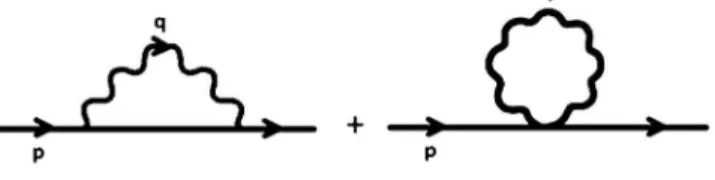
A. Meson self-energy

The first self-energy function that we evaluate here is the one from the mesonic sector. This quantity corresponds to the diagrams presented in the Fig. 1. In order to avoid repetition, in the calculation throughout this section it is rather interesting to show explicitly some details common for all radiative functions only in this first discussion.

Further, from the definition (32), it follows that one can write the self-energy functionatorder as

ð1Þ_{ðpÞ ¼ ig}2ð4 !ÞZ d!q

ð2Þ!

_{ð2p qÞ}

ð2p qÞ

ðp qÞ2 _m2_þi 2

½iD_{ðqފ: (57)} FIG. 1. Meson self-energy diagrams.

4_{We have used the following decomposition:}ðRÞ_{ðpÞ ¼}ðRÞ

1 ðpÞp2þ ðRÞ 2 ðpÞ.

3_m

We can combine the terms over the same denominator, and then substituting the explicit form of the photon propagator iD_{ðqÞ, get the following expression:}

ð1Þ_{ðpÞ ¼ ig}2Z d4q ð2Þ4

_{ð2p qÞ}

ð2p qÞ 2ððp qÞ2 m2Þ

ðp qÞ2 _m2_þi

_{ð1 Þ}qq q2

₁

q2

qq

q2 _m2 P

₁

q2 _m2 P

þ q

_q

q2_ðq2 _m2 PÞ

: (58)

Actually, the first term is inherent from the usual scalar theory (ultraviolet divergent), while the other two terms are from Podolsky’s theory.5Once we have already studied the effects of Podolsky’s terms in the fermionic electrodynamics [17], our interest then relies on investigating how the second and third terms behave in order to eliminate or not the ultraviolet divergence from the theory, rendering hence a better UV behavior, and also whether they give new and interesting information.

Therefore, the above terms are evaluated following the well-known set of rules of the standard Feynman integrals and dimensional regularization [28]. Thus, for the first term in (58) we find6

ð1;1Þ_{ðpÞ ¼}

4

p24

2þ

7 6

þm22

7 2

ð1 Þ 4

p2 2 þþ

15 12

þm22

7

6

þð_fin1;1ÞðpÞ;

(59)

with¼₄g2, and¼4 !!0þ_{the ultraviolet dimensional regularization parameter.}

Following the same steps as for the previous calculation ofð1;1Þ_{, one may obtain the following expressions for the}

second term:

ð1;2Þ_{ðpÞ ¼}

4

p24

2þ

7 6

þm22

7

2

₁₄

1

2 7

m2 P

þ 4

p2

₂

þþ 15 12

þm2

₂

7

6

₄

þ 1

3 2

m2_P

þð_fin1;2ÞðpÞ; (60)

and for the third one:

ð1;3Þ_{ðpÞ ¼ ð1 2Þ}

4

p2 2 þþ

15 12

þm22

7

6

₂

þ 1

6

m2 P

þð_fin1;3ÞðpÞ: (61)

Now, by combining the above results, Eqs. (59)–(61) into Eq. (58), it follows that the regularized expression for the meson self-energy function is given by

ð1Þ_{ðpÞ ¼}

4

₁₂

2

3 6

m2 Pþ

ð1Þ

finðpÞ; (62)

where the explicit expression for the finite term,ð_fin1ÞðpÞ ¼ ð_fin1;1ÞðpÞ þ_finð1;2ÞðpÞ þ_finð1;3ÞðpÞ, is given by Eq. (B1).

Although some contributions from the m_P-dependent term eliminate the usual UV divergences (from the p2 and m2 _{terms), they also gave rise to a novel and} unex-pected gauge-independent logarithmic divergence, which

is proportional to the theory’s free parameter mP and therefore it is not present in the conventional theory. Actually, the appearance of this divergence might be dis-cussed in terms of power counting as well. Nevertheless, this can be a problematic situation, once we have the equalities between the renormalization constants to be satisfied. We will come back to this problem in Sec.VII, where it will be further discussed in detail.

B. Photon self-energy at one loop

By means of complementarity, since it has the same expression as the usual theory, we present here only the final expression of the photon self-energy function (25) at order (Fig.2):

ðkÞ ¼

4

₂

₁

3

þZ1 0 dx

ð1 2xÞ2_ln 42 m2 _{xð1 xÞk}2

; (63)

5_{We will always represent the usual contribution through the} index (1) in the radiative functions and the new contributions by (2) and (3).

with being the t’Hooft mass. Regardless its use in the discussion on the running coupling constant, this result is not relevant for our main interest, since it does not depend on Podolsky’s parameter. However, we expect to obtain new and interesting results for the two-loop expression of this self-energy function, since it will possibly depend on this free parameter. This discussion will be presented below.

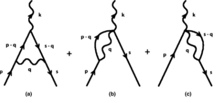
C. Vertex part

We now turn our attention to the calculation of the vertex partðp; sÞ, Eq. (35), atorder. Where, as usual, pandsare, respectively, the momenta of the incident and

emerging scalar fields, whilek¼p sis the momentum of the photon. We show the corresponding diagrams in Fig.3.

We have the contribution of three diagrams for the ðp; sÞat this order of approximation:

ðp; sÞ ¼

ðaÞ

ðp; sÞ þðbÞðpÞ þðcÞðsÞ: (64)

But, the diagramsðbÞandðcÞare related by the momentum symmetry p$s. Thereafter, we shall present the calcu-lation and expression for the diagramsðaÞandðbÞonly:

ðaÞðp; sÞ ¼ ig2ð4 !Þ

Z d!_q

ð2Þ!

_{ð2p qÞ}

ð2s qÞ

ðs qÞ2 _m2_þi

ðpþs 2qÞ ðp qÞ2 _m2_þi

½iD_{ðqފ; (65)}

and

ðbÞðpÞ ¼2ig2ð4 !Þ

Z d!_q

ð2Þ!

_{ð2p qÞ}

ðp qÞ2 _m2_þi

½iD_{ðqފ: (66)}

Due to the linear structure of the photon propagatorDthe above expressions are decomposed in a sum of three terms, likewise as happened to the meson self-energy function, Eq. (58), where the first term is the contribution from the usual scalar electrodynamics while the second and third ones are from Podolsky’s theory.

1.ðaÞ

We calculate first the contribution of the diagramðaÞ, Eq. (65), where its three terms have the following regularized expressions:

ða;1Þðp; sÞ ¼ 4

₂

1

6 ð1 Þ

₁

2

5 12

ðpþsÞþ ðfinÞða;1Þðp; sÞ; (67)

ða;2Þðp; sÞ ¼ 4

₂

1

6

₁

2

5 12

ðpþsÞþ ðfinÞða;2Þðp; sÞ; (68)

and

ða;3Þðp; sÞ ¼ ð1 2Þ 4

₁

2

5 12

ðpþsÞþ ðfinÞða;3Þðp; sÞ: (69)

Thus, summing up these results, Eqs. (67)–(69), we determine the first contribution as being finite: ðaÞðp; sÞ ¼ ðfinÞ

ða;1Þ

þ ðfinÞ

ða;2Þ

þ ðfinÞ

ða;3Þ

; (70)

where the explicit expression of the quantityðaÞ_{is given by (B4). We see thus that this quantity is already UV finite and}

independent ofby itself atorder. Now, we expect that the other two diagrams do present this same finiteness and independence.

FIG. 2. Photon self-energy diagrams.

2.ðbÞ

Now, for the contribution of the diagramðbÞ, Eq. (66), we get the following results:

ðb;1ÞðpÞ ¼ 4p

₆

3

1 3ð1 Þ

þ ðfinÞ

ðb;1Þ

ðpÞ; (71)

ðb;2ÞðpÞ ¼ 4p

₆

3

1 3

þ ðfinÞðb;2ÞðpÞ; (72)

and

ðb;3ÞðpÞ ¼ ð1 2Þ

12pþ ðfinÞ

ðb;3Þ

ðpÞ: (73)

Therefore, by combining Eqs. (71)–(73), one obtains the finite expression ðbÞðpÞ ¼ ðfinÞ

ðb;1Þ

þ ðfinÞ

ðb;2Þ

þ ðfinÞ

ðb;3Þ

; (74)

with the explicit expression of the quantityðbÞ_{given by}

ðB5Þ. We see that this quantity is also UV finite and independent ofatorder, as the previous one.

Therefore, through the symmetry property between the diagrams ðbÞ and ðcÞ, we compute the diagram ðcÞ by taking the limitp!sin Eq. (74). Thus, we have deter-mined that the contributions of these three diagrams are actually UV finite. However, we have here an apparent violation of the WFT identities, once we do have the presence of a novel UV divergence in the resulting expres-sion of, Eq. (62), which is not present, at least, here in the vertex function. Nevertheless, we must now calculate the next vertex functionand evaluate the counterterms and only then discuss whether this violation actually does exist or not.

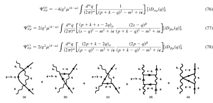
D. Vertex part

The last subject to be discussed in this section, before the analysis upon the renormalizability of GSQED4, is the calculation of the vertex part , Eq. (37), which is related to Compton’s scattering. The five diagrams that contribute to this function at order are shown in the Fig.4.

The contributions for the vertex part (37) atorder are given by the sum of terms

ðp; k;s; k1Þ ¼ ðaÞþ ðbÞþ ðcÞ þ ðdÞþ ðeÞ;

(75)

where the explicit expression of each contribution has the following form:

ðaÞ

¼ 4ig2ð4 !Þ

Z d!_q

ð2Þ!

₁

ðpþk qÞ2 _m2_þi

;½iDðqފ; (76)

ðbÞ

¼2ig2ð4 !Þ

Z d!_q

ð2Þ!

_{ðpþkþs 2qÞ}

ðs qÞ2 _m2_þi

ð2s qÞ

ðpþk qÞ2 _m2_þi

½iDðqފ; (77)

ðcÞ

¼2ig2ð4 !Þ

Z d!q

ð2Þ!

_{ð2pþk 2qÞ}

ðp qÞ2 _m2_þi

ð2p qÞ

ðpþk qÞ2 _m2_þi

½iDðqފ; (78)

ðdÞ

¼ ig2ð4 !Þ

Z d!_q

ð2Þ!

_{ð2pþk 2qÞ}

ðpþk qÞ2 _m2_þi

ðpþkþs 2qÞ

ðs qÞ2 _m2_þi

ð2s qÞ_{ð2p qÞ}

ðp qÞ2 _m2_þi

½iDðqފ; (79)

and

ðeÞ

¼2ig2ð4 !Þ

Z d!q

ð2Þ!

₁

ðp qÞ2 _m2_þi

ð2p qÞð2s qÞ ðs qÞ2 _m2_þi

½iD_{ðqފ: (80)}

Despite the fact that each one of the contributions of vertex part can be written as the sum of three terms, we shall present directly their final expressions, as we did for the previous radiative functions. We also have that the contributionðcÞ can be evaluated through the expression ofðbÞby taking the limitss!pand$.

1.ðaÞ

The first contribution evaluated is from diagramðaÞ, Eq. (76). We have the following regularized result:

ða;1Þ

¼

4

₈

4

ð1 Þ

₂

þ ð _finÞða;1Þ; (81)

ða;2Þ

¼

4

₈

4

₂

þ ð finÞða;2Þ; (82)

and

ða;3Þ

¼ ð1 2Þ

4

₂

þ ð _finÞða;3Þ: (83)

Thus, by combining the Eqs. (81)–(83), it follows that

ðaÞ

¼ ð finÞða;1Þþ ð finÞða;2Þþ ð finÞða;3Þ; (84)

with the finite term ðaÞgiven by Eq. (B9).

2.ðbÞ andðcÞ

Now, evaluating the contribution of the diagramðbÞ, Eq. (77), we get the following results:

ðb;1Þ

¼

4

₂

ð1 Þ

₂

1 3

þ ð _finÞðb;1Þ; (85)

ðb;2Þ

¼

4

₂

₂

1 3

þ ð _finÞðb;2Þ; (86)

and

ðb;3Þ

¼ ð1 2Þ

4

₂

1 3

þ ð _finÞðb;3Þ: (87)

We find collecting Eqs. (85)–(87), the finite expression

ðbÞ

¼ ð finÞðb;1Þþ ð finÞðb;2Þþ ð finÞðb;3Þ; (88) where ðbÞis given by Eq. (B10). The resulting contribution of ðcÞ, Eq. (78), is also given by the finite expression (B10), where the appropriated limitss!pand$have to be carefully taken.

3.ðdÞ

Next, for the contribution of the diagramðdÞ, Eq. (79), one obtains

ðd;1Þ

¼

4

₂

1 3

ð1 Þ

₄

3 2

3 5 9

ðd;2Þ

¼

4

₂

1 3

₄

3 2

3 5 9

þ ð _finÞðd;2Þ; (90)

and

ðd;3Þ

¼ ð1 2Þ

4

₄

3 2

3 5 9

þ ð _finÞðd;3Þ: (91)

By combining Eqs. (89)–(91), we get the expression

ðdÞ

¼ ð finÞ

ðd;1Þ

þ ð finÞ

ðd;2Þ

þ ð finÞ

ðd;3Þ

; (92)

with the finite term ðdÞgiven by Eq. (B11).

4.ðeÞ

The last contribution to be evaluated is that corresponding to diagramðeÞ, Eq. (80), which yields to

ðe;1Þ

¼

4

₄

1 2

þ ð1 Þ

₄

5

3 2

þ ð _finÞðe;1Þ; (93)

ðe;2Þ

¼

4

1 4

þ2

₄

5

3 2

þ ð _finÞðe;2Þ; (94)

and

ðe;3Þ

¼ ð1 2Þ

4

₄

5

3 2

þ ð _finÞðe;3Þ: (95)

Finally, summing Eqs. (93)–(95), one obtains

ðeÞ

¼ ð finÞðe;1Þþ ð finÞðe;2Þþ ð finÞðe;3Þ; (96)

where the finite term ðeÞis given by Eq. (B12).

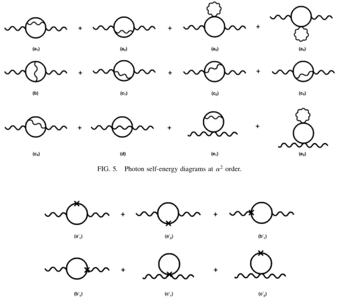
From the above results for the radiative correction ex-pressions at order, we see that the primitive divergent self-energy diagrams are only from the meson and photon self-energy functions, Eqs. (62) and (63), respectively. As a matter of fact, to elucidate this last point, we shall present next a discussion upon the photon self-energy at2 _order, which has contributions from the meson, and three-point and four-point vertex functions. However, we will find another primitive divergence on the photon self-energy, but nowmPdependent.

E. Photon self-energy at two loops

In comparison with the usual theory and also with GQED₄, the GSQED₄ presents an unexpected novel divergent structure. In this sense, it is important to supply the discussion of this new kind of divergence (m_P-dependent one), present in the electron self-energy Eq. (62), with new information and details. Therefore, for this purpose, we will present a diagrammatic analysis on the results of2_{-order photon self-energy. Our interest in} this particular function is driven mainly by the divergence structure embedded on it from the meson self-function [the set of diagrams ðaÞ and ðeÞ]. Furthermore, we are motivated to present also a discussion on the behavior of this self-energy function in the light of the higher-order

terms, once the -order calculation is not sensitive to these effects.

The diagrams presented in this order are depicted in Fig.5and the counterterm diagrams in Fig.6. It is worth stressing that we do not have the intention of presenting here a formal proof concerning the complete renormaliz-ability of the theory. Nevertheless, we believe that a quali-tative discussion does provide all the necessary information concerning the renormalizability of the theory, especially regarding them_P-dependent divergent diagrams.

First, as it is easily seen, we do have that the set of diagramsðaÞandðeÞare contributions that come from the meson self-energy . It is not difficult to show through their divergent structure that the diagrams ðaÞ and ðeÞ are UV divergent, being m_P dependent (here the other divergences are also canceled as the previous self-energy functions) and, as it turns out, they are absorbed by the counterterm diagramsða0

1Þ,ða02Þ, andðc02Þ.

Next, we do have that the set of diagrams ðbÞ andðcÞ carry contribution from the three-point vertex . Thus, after a calculation one obtains that the diagrams ðbÞ and ðcÞ contain an m_P-dependent UV divergence—a diver-gence that is absorbed by the counterterm diagrams ðb0

1Þ andðb0

2Þ.

primitive divergence of the photon self-energy diagram, and them_P-dependent ultraviolet divergence presented in this diagram is absorbed by the counterterm diagramðc0

1Þ. With the above results, we see that no further counterterms are needed; therefore, the renormalizability of the theory is consistently stated.

VII. RENORMALIZED QUANTITIES

In this section we finally present the explicit expressions and discussion on some renormalized quantities. We start by presenting the expressions for the counterterms evaluated atorder. Also, from the counterterms expres-sions we will be able to recognize that the novel logarith-mic divergence present at the meson self-energy, Eq. (62), actually does not spoil the WFT identities, once it is removed by the mass counterterm Z0. Afterwards, we discuss the effective coupling of the GSQED₄ and its relation with the GQED₄ as well. Furthermore, from the

running coupling constant expression we will be able to determine a energy range where the theory is well defined.

A. Counterterms expressions

1._Z3

First, we have the simplest counterterm expression at order, which is computed from the condition (50) and result (63); in this way it follows that

ðZ₃ 1Þð1Þ_¼

12

₂

þln

₄2

m2

; (97)

showing that the ultraviolet divergence of the photon propagator is absorbed properly by its counterterm.

2._Z 0

Next, we compute the expression for the counterterm Z0 through the condition (54) and expression (62), and it follows for b¼m2P

m2>4the expression

FIG. 6. Photon counterterms diagrams at2_order.

ð_Z1Þ 0 ¼

4

₁₂

2

3 6þ13 ln

₄2

m2

_m2 P m2

þ 2

ð 3Þ _IR þ

24f144b

3_þ126b2_{ð1 4Þ þ2bð99þ14Þ 6g}

þ 4

12b4_þ3 2b

3_{ð40 7Þ þb}2_{ð20 66Þ þb6} 3

2

þ 3

logðbÞ

þ 8

b

ffiffiffiffiffiffiffiffiffiffiffiffiffiffiffiffiffiffi

bðb 4Þ

p ð24b4 21b3ð8 1Þ þb2ð324 82Þ

3bð44 5Þ þ20Þ

2

4log

_{b 2þ}pffiffiffiffiffiffiffiffiffiffiffiffiffiffiffiffiffiffi_{ðb 4Þb}

b 2 pffiffiffiffiffiffiffiffiffiffiffiffiffiffiffiffiffiffiðb 4Þb

þlog

_b pffiffiffiffiffiffiffiffiffiffiffiffiffiffiffiffiffiffi_{ðb 4Þb}

bþpffiffiffiffiffiffiffiffiffiffiffiffiffiffiffiffiffiffiðb 4Þb

3

5: (98)

Otherwise, the logarithm must be replaced by an arctan function. We have introduced the infrared dimensional parameter asIR¼! 4,IR!0 . Finally, as it turns out, we see explicitly in the above expression, Eq. (98), that the novel mP-dependent logarithmic divergence of the meson propagator is actually absorbed by the countertermZ0. Therefore this divergence poses no harm to the theory’s renormalizability, once the gauge WFT identities are still satisfied.

3._Z2

At last, we compute_Z2 through (53) and (62). Thus, under the conditionb¼m2P

m2>4it follows that

ð_Z1Þ 2 ¼

2

ð 3Þ _IR þ

2400ð720b

4_{ð2 1Þ þ60b}3_{ð81 202Þ þ30b}2_{ð858 19Þ 20bð9þ577Þ þ741}

1482Þ

80ð12b

5_{ð2 1Þ þb}4_{ð99 238Þ þ2b}3_{ð353 59Þ b}2_{ð668þ51Þ þ10bð13 6Þ}

þ20ð3 ÞÞlog½bŠ þ 80

b

ffiffiffiffiffiffiffiffiffiffiffiffiffiffiffiffiffiffi

bðb 4Þ

p ð12b5ð2 1Þ þb4ð123 286Þ þ2b3ð567 146Þ

þ5b2_{ð7 340Þ þ2bð1þ383Þ þ40ð1 ÞÞ}

2

4log 2

4b

ffiffiffiffiffiffiffiffiffiffiffiffiffiffiffiffiffiffi

bðb 4Þ

p

bþpffiffiffiffiffiffiffiffiffiffiffiffiffiffiffiffiffiffibðb 4Þ

3

5þlog 2

4bþ

ffiffiffiffiffiffiffiffiffiffiffiffiffiffiffiffiffiffi

ðb 4Þb

p

2 b pffiffiffiffiffiffiffiffiffiffiffiffiffiffiffiffiffiffiðb 4Þb 2

3

5 3

5: (99)

Such an expression is also an ultraviolet finite quantity at order.

Actually, by computing the counterterms Z1 and Z4 through the conditions (55) and (56), respectively, we obtain, for both quantities, the same expression as (99) at order. Therefore, such results are in agreement with the gauge WFT identities, and despite the fact that the meson propagator presents an unexpected divergence, it was shown that it is suitably absorbed by its proper counterterm. We also observe that the above counterterms expressions, (98) and (99), are also infrared finite at the Fried-Yennie gauge choice, ¼3 [29]. Therefore, with these results we see that the renormalizability ofGSQED₄ is attained (even to the two-loop photon self-energy re-sults) and the divergences are consistently absorbed by the appropriated counterterms.

B. Effective coupling constant

Although the renormalization constantZ3 expression at order, Eq. (97), does not feel the effects from the higher-order terms, there are other quantities that may present modifications from the usual expression at this order. One of these quantities is the Born amplitude [19]. Actually, this renormalized amplitude depends on Z₃, which

provides a suitable context for our discussion. Also, from this analysis we will be able to introduce an invariant quantity, the so-called running coupling constant for the GSQED₄, and from the later, we shall determine an energy range for the theory.

By means of simplicity, we will work in the Landau gauge¼0. Therefore, from the photon propagator, in the Born scattering andk2 _m2_{regime, one can define in this} approximation the running coupling constant as

_Rðk2_{Þ ¼1þ1} 1 k2 _m2

P

12

₂

þln

₄2

m2

þ 12ln

_k2

m2

;

for which it can immediately be casted as

_Rðk2_{Þ ¼} Rðm2Þ

1þRðm 2_Þ

12 1 1 k2

m2 P

ln

_k2

m2

; (100)

where_Rðm2_{Þ ¼Z}

Nevertheless, further modifications to the Born scatter-ing can also be studied in subsequent orders of perturbation theory. Thus, in order to obtain these higher-orders mod-ifications, we can sum an important class of diagrams, which consists in the most divergent set of logarithms. Therefore, the running coupling constant expression, in such a regime and approximation, can be cast in the following form:

1 _Rðk2_Þ¼

1 _Rðm2_Þ

1 12

1 1 k2

m2 P

ln

_k2

m2

: (101)

Exactly as it happens in the usual scalar theory in relation to the QED, the rate of change of the coupling constant in GSQED4 is one-fourth of that fromGQED4 [18]. Also, we see the presence of a pole atm2

P¼k2on its expression; and, in comparison to theSQED4 expression [19] it provides a validity regime: m2_k2_{< m}2

P, where the generalized theory is in fact well defined.

VIII. CONCLUDING REMARKS

Despite the spinless aspect of generalized scalar electrodynamics, our present analysis has provided in-sights of a particular HD term in an interesting field theory, when the GSQED4 is discussed in the context of effective theories. Foremost is the role played by the HD and the generalized gauge condition as well, that showed significant importance when the radiative correc-tions were computed at order. Also, the presence of a new type of divergence in the mesonic sector is a result of some interest in itself.

In this paper, we presented a proper study regarding the complete quantization and consistent renormalization, and subsequent consequences, of the generalized scalar electrodynamics. The first part of this article was devoted to the formal development of GSQED4. After we con-structed the transition amplitude through the Batalin-Fradkin-Vilkovisky covariant method, we derived by functional methods the four fundamental Green’s func-tions for the theory and the Ward-Fradkin-Takahashi identities as well. And, our main motivation here relied on observing the theory’s behavior upon these m_P-dependent terms, once the scalar theory possessed a more interesting interacting structure. It was also shown that the two gauge WFT identities, Eqs. (44) and (45), were of high importance on the discussion regarding the renormalizability of GSQED₄. On the discussion about the renormalizability of GSQED4 we made use of a previous result on the renormalization condition for the photon propagator [18].

In the second part of the article, the calculation of radiative corrections took place, and we presented there the evaluation and discussion of the results of the self-energy functions and counterterms atorder. We initially discussed the results on the meson self-energy, where we

found that the massive terms canceled the usual ultravio-let divergences but also generated a novel logarithmic divergence, which is proportional to the free parameter m_P and therefore not present in the conventional theory. However, for the vertex parts and it was found that the massive contribution of the photon propagator can-celed out all the divergences, resulting, thus, in an ultra-violet finite expression for both quantities. Moreover, once the massive contributions were not presented in the photon self-energy atorder, we provided a diagram-matic discussion about the contribution of the diagrams in 2 _{order and its counterterms, where we also found} m_P-dependent divergence; but all of them are properly absorbed by the theory’s counterterms. Next, we pre-sented the explicit expressions for the counterterms at order. Actually, we have shown that the m_P-dependent divergence from the meson self-energy function was ab-sorbed suitably by_Z0; showing, therefore, that the gauge WFT identities (Z1 ¼Z2 ¼Z4) are still satisfied at this order. Also, the expressions for the counterterms, _Z

0, _Z2, _Z1, and_Z4, are infrared finite at the Fried-Yennie gauge, ¼3. Lastly, from the effective coupling expres-sion we found an energy scale,m2 _k2_{< m}2

P, where the generalized theory is in fact well defined.

Once again, Podolsky’s theory has shown to possess a richness of features, and be interesting in its own right. Here we have successfully studied the generalized elec-trodynamics of spinless charged particles in rich detail. Furthermore, with these results we now have good in-sights to deal also with non-Abelian fields, for instance, since the scalar theory shares some general properties with the non-Abelian one [30]. However, this study might take place not only in a four-dimensional space-time, but also in different dimensionality, since the field theories in lower dimensions are again receiving attention nowadays. Currently, based on the present results, the authors are also investigating the scalar generalized electrodynamics also at a thermodynamical equilibrium. An interesting and still unexplored issue that we think deserves attention next is the study of scattering processes with external fields of Podolsky’s theory, either in the context of spinor or scalar electrodynamics [31]. These issues and others will be further elaborated, investigated, and reported elsewhere.

ACKNOWLEDGMENTS

The authors thank the referee for the comments and suggestions, and Daniel Soto Barrientos for the fruitful discussions. R. B. thanks FAPESP for full support and B. M. P. thanks CNPq and CAPES for partial support.

APPENDIX A: FUNCTIONAL QUANTITIES

ð1Þðx; h;zÞ ¼g

Z

d4_wd4_{rSðr; hÞ}

ðw; r;zÞSðx; wÞ; (A1)

and

ð2Þðx; h;zÞ ¼ g2

Z

d4wd4vd4rd4g1d4u½Sðg1; hÞDðx; uÞ ðr; g1;uÞSðv; rÞ ðw; v;zÞSðx; wÞ

þSðv; hÞ ðw; v;zÞSðg₁; wÞD_{ðx; uÞ}

ðr; g1;uÞSðx; rފ

þig2Z _d4_wd4_vd4_{uSðv; hÞD}

ðx; uÞðw; x;z; uÞSðx; wÞ: (A2)

Also, in the definition of meson self-energy, Eq. (32), we have introduced ð3Þðz; y; hÞ ¼g

Z

d4_sd4_{fSðs; yÞD}

ðf; hÞ ðz; s;fÞ; (A3)

and

ð4Þðz; y; h; xÞ ¼ g2

Z

d4rd4vd4fd4cd4u½Sðc; yÞD_{ðu; xÞ}

ðr; g;uÞSðv; rÞDðf; hÞ ðz; v;fÞ

þSðv; yÞD_{ðf; hÞ}

ðr; v;fÞSðc; rÞDðu; xÞ ðz; g;uފ

þig2Z d4vd4fd4uSðv; yÞD_{ðf; hÞDðu; xÞ}

ðz; v;f; uÞ: (A4)

Furthermore, in the definition of vertex functions and , Eqs. (35) and (37), respectively, we have introduced the quantities 5 11, which are actually lengthy, and their derivation and content do not add anything to the formal development of the theory. Also, all of them can be computed by following the standard guideline of functional methods presented here. Thus, we have their definitions read as

ð5Þðx; y; h; zÞ ¼

Z

d4_w 2 ’ðyÞ’y_ðwÞ

J_ðhÞ

AðzÞ

2_W

ðwÞðxÞ

; (A5)

ð6Þðx; y; zÞ ¼lim_h!x

t!x

Z

d4_w 2 ’ðyÞ’y_ðwÞ

2 J_ðtÞJðhÞ

AðzÞ

2_W

ðwÞðxÞ

; (A6)

ð7Þðx; y; zÞ ¼2i

Z

d4_w 2 ’ðyÞ’y_ðwÞ

AðzÞ

3_W

J_{ðxÞðwÞðxÞ}

; (A7)

ð8Þðx; y; sÞ ¼lim h!x

ð7Þðx; y; hÞ; (A8)

gð9Þ ðx; y; z; s; hÞ ¼

Z

d4_w 2 ’ðyÞ’y_ðwÞ

J_ðhÞ

AðsÞ

AðzÞ

2_W

ðwÞðxÞ

; (A9)

ð10Þðx; y; z; sÞ ¼lim_f!x h!x

Z

d4_w 2 ’ðyÞ’y_ðwÞ

JðfÞ

J_ðhÞ

AðsÞ

AðzÞ

2_W

ðwÞðxÞ

; (A10)

and

ð11Þðy; z; sÞ ¼lim f!x h!x

Z

d4_w 2 ’ðyÞ’y_ðwÞ

AðsÞ

AðzÞ

2_W

JðfÞJ_ðhÞ

: (A11)

Also, within the formal development, and in the above quantities as well, we have used the following definitions for the connected two-point functions:

iDðx; yÞ ¼ 2_W

JðyÞJðxÞ

s¼0