Brazilian Journal of Physics, vol. 35, no. 4B, December, 2005 1041
Phase Space Solutions in Scalar-Tensor Cosmological Models
Jos´e C. C. de Souza
Departamento de F´ısica Matem´atica, Instituto de F´ısica, Universidade de S˜ao Paulo, C.P. 66318, 05315-970 S˜ao Paulo, SP, Brazil
and Alberto Saa
Departamento de Matem´atica Aplicada, IMECC – UNICAMP, C.P. 6065, 13083-859 Campinas, SP, Brazil (Received on 15 October, 2005)
An analysis of the solutions for the field equations of generalized scalar-tensor theories of gravitation is performed through the study of the geometry of the phase space and the stability of the solutions, with special interest in the Dicke model. Particularly, we believe to be possible to find suitable forms of the Brans-Dicke parameterωand potential V of the scalar field, using the dynamical systems approach, in such a way that they can be fitted in the present observed scenario of the Universe.
I. SCALAR-TENSOR THEORIES OF GRAVITATION
In a homogeneous and isotropic space, described by the Friedmann-Lematre-Robertson-Walker metric
ds2=−dt2+a2(t) "
dr2 1−Kr2+r
2(dθ2+
sin2θdϕ2) #
, (1)
whereais the scale factor andKis the spatial curvature index, gravitation can be described by an action of the kind
S= 1 16π
Z d4√−g
·
φR−ω(φφ)gab∇aφ∇bφ−V(φ)
¸
+Sm, (2)
whereSm is the action of usual matter, g is the determinant of the metric tensor,ωis a coupling function (which we will eventually assume to be a constant, known as Brans-Dicke parameter) andV(φ)is the potential of the scalar fieldφ[2].
From (2), we obtain for the field equations:
H2=−H µφ˙
φ 
+ω 6
µφ˙ φ
¶2
+V6φ(φ)−K a2+
8πρm 3φ , (3)
˙
H = −ω 2
µφ˙ φ
¶2 +2H
µφ˙ φ
+ 1
2(2ω+3)φ ·
φddφV −2V+dωdφ(φ˙)2 ¸
+K
a2− 8π
(2ω+3)φ[(ω+2)ρ
m+ωPm], (4)
¨ φ+
µ
3H+ 1 2ω+3
dω dφ
¶ ˙
φ = 1
2ω+3 ·
2V−φdV dφ+ 8π(ρm−3Pm)], (5) whereH≡a/a˙ is the Hubble parameter andρmandPmare the energy density and the pressure of the material fluid.
As usual, we parameterize the equation of state for the fluid asPm= (γ−1)ρmwithγa constant chosen to indicate a va-riety of fluids that are predominantly responsible for the ergy density of the Universe. We can see that through the en-ergy conservation equation ˙ρm+3H(ρm+Pm) =0 we obtain ρm=ρ
0/a3γ, withρ0a constant.
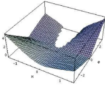
FIG. 1: Upper sheet of the of the phase space for a model withω=10 (Brans-Dicke), corresponding to the positive sign in eq. (7) [2]. The “hole” in the surface indicates the region forbidden for the orbits of the solutions.
II. THE CASE FORV=12m2φ2ANDK=0
In the referred paper [2], the author proceeds to show the phase space allowed for the orbits of solutions for these field equations in several cases with different potentials and para-meters ω. For example, in the case of vacuum, flat space (K=0) and potentialV=12m2φ2, equation (3) was rearranged as (makingm≡1)
ωφ˙2
−6Hφφ˙+ (1 2φ
2
−6H2φ)φ=0, (6) which has the solutions
˙
φ±(H,φ) =ω1 "
3Hφ± r
3(2ω+3)H2φ2−1
2ωφ
2
# . (7)
The assumption of flat space is required in order to reduce the dimensionality of the phase space.
We want to analyze qualitatively the geometry of the phase space(H,φ,φ˙), expecting to infer the form of the functions ω(φ)andV(φ)to fit better the available data on the structure of the Universe.
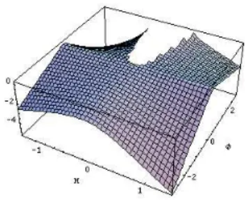
The phase space for this situation is composed of a 2-d sur-face with two sheets, related to the lower and upper signs in eq. (7). Figures 1-3 show the phase space for the choice ω=10.
The fixed points for this dynamical system, obtained mak-ing ˙H = φ˙ = 0, are de Sitter solutions, given by H0 =
1042 Jos´e C. C. de Souza and Alberto Saa
FIG. 2: Lower sheet of the phase space, now corresponding to the negative sign in eq. (7).
FIG. 3: The complete phase space composed of the upper and lower sheets linked to each other at the boundary of the forbidden region.
III. THE CASE FORV=ΛφANDK=0
Following other works ([3]-[5]) which give a complete analysis of the phase space for Brans-Dicke model with a cos-mological constantΛ (simply makingV(φ) =Λφin the ac-tion), we can illustrate the situation in which ω has a very large value andγ=0. Therefore, the energy density of the fluid is a constant ρ0. It should be emphasized that recent
observational and simulation results seem to favor a scenario very similar to this one ([6],[11]-[14]). The solutions in this case are written as
˙
φ±(H,φ) =
1 ω ·
3Hφ±
q
9H2φ2−ω[φ2(Λ−6H2) +16πρ 0]
¸ . (8)
With this solutions, we are able to show the phase space for a particular choice of constantsΛ,ωandρ0.
We proceed to find the dynamical equations system for this simple model, as done before.
Naming∆the expression under the root in eq.(8), we can write the equation for ˙H:
˙
H± = −2ωφ1 2
h
3Hφ±√∆i2+2ωH "
3H± √
∆ φ
#
− 1
2(2ω+3) µΛ
2 + 16πρ0
φ 
. (9)
Now, equations (8) and (9) form the system for which the fixed points are the solutionsH0=±
q
8πρ0/3φ20+Λ/6 .
Of special interest is the search for the most adequate func-tionsω(φ)andV(φ), that may be more complicated than what was assumed until here.
FIG. 4: Complete phase space for a Brans-Dicke model with a cos-mological constantΛ=1, energy densityρ0=2 and constant
para-meterω=50000, showing two sheets linked by the boundary of the forbidden region, as in the precedent case.
IV. CONCLUSIONS
The method of analyzing the geometry of the phase space have proved to be a useful tool in the search for the solutions of the field equations of generalized gravity models. Our aim is to achieve a complete analysis of the simple model pre-sented before (including the stability of the solutions, via Lya-punov’s direct method [1], in order to investigate further its attraction basin) and to apply more sophisticated functions to it.
V. ACKNOWLEDGMENTS
This work is supported by Conselho Nacional de Desen-volvimento Cient´ıfico e Tecnol´ogico (CNPq). We would like to thank F. C. Carvalho for useful discussions.
[1] J. LaSalle and S. Lefschetz, Stability by Lyapunov’s Direct Method. Academic Press (1967)
[2] V. Faraoni, Annals of Physics317, 366 (2005)
[3] S. J. Kolitch, Annals of Physics246, 121 (1996) [4] S. J. Kolitch, Annals of Physics241, 128 (1995)
Brazilian Journal of Physics, vol. 35, no. 4B, December, 2005 1043
[6] A. G. Sanchez et al., astro-ph/0507583
[7] G. Esposito-Farse and D. Polarski, Phys. Rev. D63, 063504 (2001)
[8] A. Saa et al., Phys. Rev. D63067301 (2001); Int. J. Theor. Phys. 40, 2295 (2001); L.R. Abramo, L. Brenig, E. Gunzig, and A. Saa, Phys. Rev. D67, 027301 (2003); gr-qc/0305008.
[9] J. D. Barrow and J. P. Mimoso, Phys. Rev. D50(6), 3746 (1994) [10] F. C. Carvalho and A. Saa, Phys. Rev. D70, 087302 (2004)
[11] G. Esposito-Farse, gr-qc/0409081
[12] B. Bertotti, L. Iess, and P. Tortora, Nature425, 374 (2003) [13] V. Acquaviva, C. Baccigalupi, S. M. Leach, Andrew R. Liddle,
and F. Perrotta, astro-ph/0412052