FORMULAC
¸ ˜
OES E ALGORITMOS BASEADOS
EM PROGRAMAC
¸ ˜
AO LINEAR INTEIRA PARA
O PROBLEMA QUADR ´
ATICO DA ´
ARVORE
DILSON LUCAS PEREIRA
FORMULAC
¸ ˜
OES E ALGORITMOS BASEADOS
EM PROGRAMAC
¸ ˜
AO LINEAR INTEIRA PARA
O PROBLEMA QUADR ´
ATICO DA ´
ARVORE
GERADORA M´INIMA
Tese apresentada ao Programa de P´os--Gradua¸c˜ao em Ciˆencia da Computa¸c˜ao do Instituto de Ciˆencias Exatas da Universi-dade Federal de Minas Gerais como requi-sito parcial para a obten¸c˜ao do grau de Doutor em Ciˆencia da Computa¸c˜ao.
Orientador: Alexandre Salles da Cunha
DILSON LUCAS PEREIRA
FORMULATIONS AND ALGORITHMS BASED
ON LINEAR INTEGER PROGRAMMING FOR
THE QUADRATIC MINIMUM SPANNING
TREE PROBLEM
Thesis presented to the Graduate Program in Computer Science of the Universidade Federal de Minas Gerais in partial fulfill-ment of the requirefulfill-ments for the degree of Doctor in Computer Science.
Advisor: Alexandre Salles da Cunha
Fichi citilográfici eliboridi peli Biblioteci do ICEx - UFMG Pereira, Dilson Lucas
P436f Formulations and Algorithms Based on Linear Integer Programming for the Quadratic Minimum
Spanning Tree Problem / Dilson Lucas Pereira — Belo Horizonte, 2014
xviii, 97 f.: il.; 29 cm.
Tese (doutorado) - Universidade Federal de Minas
Gerais – Departamento de Ciência da Computação.
Orientador: Alexandre Salles da Cunha
1. Computação - Teses. 2. Programação (Matemática) - Teses. 3. Programação inteira - Teses.
3. Lagrange, funções de - Teses. I. Orientador. II. Título
Agradecimentos
O desenvolvimento deste trabalho s´o foi poss´ıvel gra¸cas `a contribui¸c˜ao de diversas pessoas:
Minha esposa, que sempre esteve ao meu lado, com seu amor, carinho e dedica¸c˜ao. Meus pais e meu irm˜ao, que sempre me deram todo o suporte e incentivo.
O Professor Alexandre, que me orientou com muito empenho, sempre se preocupou com que eu pudesse atingir uma boa forma¸c˜ao, e me forneceu in´umeras li¸c˜oes, nos mais diferentes aspectos.
Os respons´aveis pelo PPGCC, que me deram a oportunidade, e que se dedicam em manter o alto n´ıvel do programa.
As secret´arias do DCC, que sempre me atenderam com prestatividade e paciˆencia. O CNPq e a CAPES, que forneceram o suporte financeiro para que eu pudesse realizar este trabalho.
A todos estes, meus sinceros agradecimentos.
Acknowledgements
Part of the research reported in this thesis was conducted while I was under the su-pervision of Michel Gendreau, at CIRRELT, Montreal - Canada. I stayed in Montreal for one year as a visiting student from the sandwich doctorate program of the Brazil-ian agency Coordena¸c˜ao de Aperfei¸coamento de Pessoal de N´ıvel Superior (CAPES). I would like to thank Michel for his hospitality and for taking his time so that we could have many valuable meetings.
Abstract
The quadratic minimum spanning tree problem (QMSTP) is an NP-Hard problem that consists of finding a spanning tree of quadratic minimum cost of a graph. In this problem, besides a cost for each edge, the objective function also involves interaction costs for each pair of edges in the tree. In a particular case of QMSTP, the adjacent-only QMSTP (AQMSTP), interaction costs are defined adjacent-only for adjacent edges. Despite having a particular cost structure, AQMSTP is as hard as QMSTP, in theory and in practice. We address both problems in this thesis.
For the general case, we first propose a linear integer programming (IP) formula-tion based on the reformulaformula-tion-linearizaformula-tion technique (RLT). This formulaformula-tion is by itself stronger than previous ones in the literature. Additionally, we also introduce a novel type of formulation. It stems from the idea of partitioning spanning trees into forests of a given fixed size. This idea yields a hierarchy of formulations of increasing strength. The larger the forests, the stronger the formulation. At the first hierarchy level, where the forests have the minimum possible size, i.e., they involve only one edge, we have precisely the RLT formulation. At the opposite end, where the forests have the maximum possible size, i.e., they are spanning trees, we have a formulation whose linear programming (LP) relaxation bound matches the optimal QMSTP solu-tion value. Many possible relaxasolu-tions of the hierarchy are studied. We give results with respect to the strength of their LP bounds and the difficulty of computing them. On the computational side, three Lagrangian relaxation (LR) procedures and two parallel branch-and-bound (BB) algorithms are developed. For the first time, several instances in the literature are solved to optimality, including some with 50 vertices.
Although successful for some types of problem instances, this general approach fails to appropriately address AQMSTP. This fact motivates an AQMSTP formulation that exploits its particular cost structure: We use the stars of the graph to formulate the problem as an IP that involves exponentially many rows and columns. We also consider a reformulation that arises by projecting the stars out of this formulation. The reformulation, although defined on a compact variable space, has exponentially
variables and large number of constraints, through separation callbacks. This facilitates the development of a BB algorithm.
In order to solve the LP relaxation of our AQMSTP formulation, we propose a row-and-column generation (RCG) algorithm. A cutting plane (CP) algorithm is proposed to solve the LP relaxation of its projection. We then develop a branch-and-cut-and-price (BCP) algorithm, based on RCG, and a branch-and-cut algorithm (BC), based on CP. Computational results show that the LP relaxation bounds provided by the AQMSTP formulation dominate the RLT based bounds we developed for the general QMSTP. As a consequence, instances with as many as 50 vertices are solved to proven optimality.
Resumo
O problema quadr´atico da ´arvore geradora m´ınima (QMSTP) ´e um problema NP-Dif´ıcil que consiste em encontrar uma ´arvore geradora de custo quadr´atico m´ınimo em um grafo. Neste problema, al´em de um custo para cada aresta, a fun¸c˜ao objetivo tamb´em involve custos de intera¸c˜ao para cada par de arestas na ´arvore. Em um caso particular do QMSTP, o QMSTP s´o com custos de adjacˆencia (AQMSTP), custos de intera¸c˜ao s˜ao definidos somente para arestas adjacentes. Apesar desta estrutura de custo particular, o AQMSTP ´e t˜ao dif´ıcil quanto o QMSTP, na teoria e na pr´atica. Ambos os problemas s˜ao abordados nesta tese.
Para o caso geral, primeiramente propomos uma formula¸c˜ao de programa¸c˜ao linear inteira (IP) baseada na t´ecnica de reformula¸c˜ao-lineariza¸c˜ao (RLT). Esta for-mula¸c˜ao ´e por si s´o mais forte que formula¸c˜oes anteriores na literatura. Adicionalmente, tamb´em introduzimos um novo tipo de formula¸c˜ao, que parte da id´eia de particionar ´arvores geradoras em florestas de um dado tamanho fixo. Esta id´eia leva `a uma hier-arquia de formula¸c˜oes cada vez mais fortes. Quanto maiores as florestas, mais forte a formula¸c˜ao. No primeiro n´ıvel da hierarquia, onde as florestas tˆem o menor tamanho poss´ıvel, i.e., envolvem apenas uma aresta, temos precisamente a formula¸c˜ao RLT. No lado oposto, onde as florestas tˆem o maior tamanho poss´ıvel, i.e., s˜ao ´arvores gerado-ras, temos uma formula¸c˜ao cujo limite da relaxa¸c˜ao de programa¸c˜ao linear (LP) tem o mesmo valor que a solu¸c˜ao ´otima do QMSTP. Diversas poss´ıveis relaxa¸c˜oes da hierar-quia s˜ao estudadas. Apresentamos resultados com respeito `a for¸ca de seus limites de LP e `a dificuldade de comput´a-los. No lado computacional, trˆes procedimentos basea-dos em relaxa¸c˜ao lagrangeana (LR) e dois algoritmos branch-and-bound (BB) paralelos s˜ao desenvolvidos. Pela primeira vez, diversas instˆancias na literatura s˜ao resolvidas na otimalidade, incluindo algumas com 50 v´ertices.
Embora a abordagem geral obtenha sucesso em alguns tipos de instˆancias, ela n˜ao se demonstra apropriada para tratar o AQMSTP. Este fato motiva uma formula¸c˜ao para o AQMSTP que explora sua estrutura de custo particular: Usamos as estrelas do grafo para formular o problema como um IP que envolve exponencialmente muitas
de vari´aveis compacto, tem um n´umero exponencial de restri¸c˜oes adicionais. Uma de suas principais vantagens est´a no fato de que a maioria dos pacotes de otimiza¸c˜ao s˜ao capazes de lidar diretamente com modelos com um n´umero pequeno de vari´aveis e um n´umero grande de restri¸c˜oes, por meio de callbacks de separa¸c˜ao. Isto facilita o desenvolvimento de um algoritmo BB.
Para resolver a relaxa¸c˜ao de LP de nossa formula¸c˜ao do AQMSTP, propomos um algoritmo de gera¸c˜ao de linhas e colunas (RCG). Um algoritmo de planos de corte (CP) ´e proposto para resolver a relaxa¸c˜ao de LP de sua proje¸c˜ao. Ap´os isto, desenvolve-mos um algoritmo branch-and-cut-and-price (BCP), baseado em RCG, e um algoritmo branch-and-cut (BC), baseado em CP. Resultados computacionais mostram que os li-mites de LP fornecidos pela formula¸c˜ao do AQMSTP dominam os lili-mites baseados em RLT que desenvolvemos para o caso geral. Como consequˆencia, instˆancias com at´e 50 v´ertices s˜ao resolvidas na otimalidade.
Lista de Siglas
AQMSTP adjacent-only quadratic minimum spanning tree problem
BB branch-and-bound
BC branch-and-cut
BCP branch-and-cut-and-price
BQFP boolean quadric forest polytope
BQP boolean quadric polytope
CP cutting plane
GMSTP generalized minimum spanning tree problem
IP linear integer programming
LP linear programming
LR Lagrangian relaxation
MSTP minimum spanning tree problem
pDP p-dispersion problem
QAP quadratic assignment problem
QMSTP quadratic minimum spanning tree problem
RCG row-and-column generation
RLT reformulation-linearization technique
SEC subtour elimination constraint
Contents
Agradecimentos ix
Acknowledgements xi
Abstract xiii
Resumo xv
Lista de Siglas xvii
1 Introduction 1
1.1 Outline of the Thesis and Main Contributions . . . 1
1.2 Motivation . . . 4
1.3 Literature Review . . . 5
1.4 Notation . . . 8
2 The Quadratic Minimum Spanning Tree Problem 9 2.1 Formulations, Linear Programming and Lagrangian Relaxation Bounds 9 2.1.1 Lagrangian Bounds from a Partial RLT Application . . . 9
2.1.2 Lagrangian Bounds Based on the Decomposition of Spanning Trees into Forests of Fixed Size . . . 15
2.2 Branch-and-Bound Algorithms . . . 30
2.2.1 Initial Upper Bounds . . . 30
2.2.2 Lower Bounds and Node Selection . . . 30
2.2.3 Branching and Variable Selection . . . 31
2.2.4 Redistribution of the Costs of Fixed Variables . . . 31
2.2.5 Parallelization . . . 32
2.3 Computational Experiments . . . 33
2.3.1 Test Instances . . . 33
3 The Adjacent-Only Quadratic Minimum Spanning Tree Problem 39
3.1 Introduction . . . 39
3.1.1 Motivation . . . 39
3.2 An AQMSTP Formulation Based on the Stars of G . . . 40
3.3 A Branch-and-Cut-and-Price Algorithm for AQMSTP . . . 41
3.3.1 Row-and-Column Generation Algorithm for Solving the LP Re-laxation of F∗ . . . . 42
3.3.2 Solving the Pricing Problem PP(v) . . . 44
3.3.3 Branch-and-Cut-and-Price Implementation Details . . . 46
3.4 A Branch-and-Cut Algorithm for AQMSTP . . . 47
3.4.1 Projecting Out Variables t . . . 48
3.4.2 A Cutting Plane Algorithm for Solving the LP Relaxation of F∗ x 49 3.4.3 Branch-and-Cut Implementation Details . . . 53
3.5 Computational experiments . . . 54
3.6 Conclusion . . . 56
4 Future Work and the Quadratic Assignment Problem 59 5 Conclusion 65 Appendix A Separation Algorithms 67 A.1 Separation of (2.5) . . . 67
A.2 Separation of (2.11) . . . 68
Appendix B Proofs 71 B.1 Proof of Proposition 2.7 . . . 71
B.2 Proof of Proposition 2.8 . . . 74
B.3 Proof of Proposition 2.11 . . . 75
Appendix C Considerations about the Work of ¨Oncan and Punnen [35] 77
D Detailed Branch-and-Bound Results 79
Bibliography 93
Chapter 1
Introduction
Assume we are given a connected and undirected graph G = (V, E), with n = |V|
vertices and m = |E| edges, and a matrix Q = (qij)i,j∈E ≥ 0 of interaction costs
between the edges of G. The quadratic minimum spanning tree problem (QMSTP) is a quadratic 0-1 programming problem that consists of finding a spanning tree of G whose incidence vector x∈Bm minimizes the function
X
i,j∈E
qijxixj.
QMSTP is NP-Hard, as proven by Assad and Xu [7] by a reduction from the quadratic assignment problem (QAP) [26, 10]. An interesting particular case of QM-STP is that in which interaction costsqij = 0 if edgesiandj do not share an endpoint.
This case is referred to as the adjacent-only QMSTP (AQMSTP). AQMSTP was also proven NP-Hard by Assad and Xu [7], by means of a reduction from the Hamiltonian path problem. Another important particular case is that in which Q is diagonal. In this case, the objective function becomes linear, and QMSTP reduces to the mini-mum spanning tree problem (MSTP), for which several polynomial time algorithms are known [42, 27].
1.1
Outline of the Thesis and Main Contributions
The thesis is divided in 5 main chapters and 4 appendices. Below we summarize each main section and its contributions.
• Chapter 1: Introduction. We began the present chapter with the definition of the two problems addressed in the thesis, QMSTP and AQMSTP. In Section 1.2 we
give motivation for studying these two problems. The QMSTP and AQMSTP literature is reviewed in Section 1.3. Some notation used throughout the thesis is presented in Section 1.4.
• Chapter 2: The Quadratic Minimum Spanning Tree Problem. We start this chap-ter by studying for the first time a formulation derived from the reformulation linearization technique (RLT), in Section 2.1.1. We show that such a formu-lation dominates other formuformu-lations in the QMSTP literature and introduce a Lagrangian relaxation lower bounding scheme to evaluate its linear programming (LP) relaxation bounds.
In Section 2.1.2, we present a novel type of formulation for QMSTP, based on the idea of decomposing spanning trees into forests. That formulation gives a hierarchy of lower bounds of increasing strength, it has the first formulation as its weakest case. With the purpose of developing computationally practical lower bounding procedures based on it, we study possible relaxations. We show that some of the relaxations are theoretically hard to solve, but manage to give a polynomial time algorithm for a particular case, which we use to develop a Lagrangian relaxation based bounding algorithm, in Section 2.1.2.1. A different approach is taken in Section 2.1.2.2, we provide a reformulation of the hierarchy and show that an easy to solve relaxation can used in a Lagrangian framework to evaluate LP lower bounds in our hierarchy. A Lagrangian relaxation algorithm, with heuristic adjustment of multipliers, is presented.
Based on two of the lower bounding schemes developed in the preceding sections, we propose two branch-and-bound (BB) algorithms in Section 2.2. We provide computational results in Section 2.3. These results show that our lower bounds are much stronger than the bounds in the literature. As a consequence, our exact algorithms manage to solve problems with up to 50 vertices, with the help of parallel programming.
1.1. Outline of the Thesis and Main Contributions 3
AQMSTP branch-and-price algorithm. We provide computational results that validate our approach: lower bounds from the star formulation are much stronger the previous ones in the literature, including those presented in Chapter 2. As a consequence, the branch-and-price algorithm solves instances with up to 40 vertices, while the algorithms developed in Chapter 2 manage to solve instances with at most 20 vertices.
In Section 3.4 we study an unusual approach for obtaining lower bounds from extended formulations with exponentially many columns. We project the vari-ables associated to stars out of our AQMSTP formulation. That results in an AQMSTP reformulation on a compact variable space, with exponentially many constraints. To evaluate its LP bounds, we propose a cutting plane algorithm, which is also used as the basis for an AQMSTP branch-and-cut algorithm. We discuss the benefits of using the projection approach, such as easier to solve pricing problems and easier to implement exact algorithms. Surprisingly, the branch-and-cut algorithm manages to solve instances with up to 50 vertices.
• Chapter 4: Future Work - The Quadratic Assignment Problem. In this chapter we discuss some lines of research we intend to investigate in the future. In particular, we show how the hierarchy presented in Chapter 2 can be extended for QAP and discuss some possible approaches for obtaining bounds.
• Chapter 5: Conclusion. Concluding remarks are presented in this chapter.
• Appendix A Separation Algorithms. We provide polynomial time, maximum flow based, separation algorithms for some inequalities used in our RLT based formu-lation of Chapter 2.
• Appendix B: Proofs. Detailed proofs for some results in the thesis are presented in this appendix.
• Appendix C: Considerations about the Work of ¨Oncan and Punnen [35]. Some results presented in ¨Oncan and Punnen [35] conflict with some results obtained by ourselves. This led us to identify some mistakes in that work. This issue, along with evidence for the correctness of the results in this thesis, are discussed in this appendix.
1.2
Motivation
There are three main motivations for studying an NP-Hard combinatorial optimization problem. First, when studying such a problem, one might develop solution techniques and theoretical results that might be generalized or adapted for other problems, and thus become contributions for the general field of combinatorial optimization. One well known example is the case of the traveling salesman problem [14, 6].
The second reason involves real-world applications of the problem. QMSTP and AQMSTP applications can be found in the context of telecommunication, transporta-tion, and hydraulic networks [7]. Below, we describe two examples of QMSTP and AQMSTP applications in more detail.
A QMSTP application can be found in the context of wireless sensor networks. In this context, the communication between sensor nodes occurs by means of radio trans-mission. Assuming that the radio frequency assigned for each possible communication link in the network has been defined beforehand, one might wish to find a communi-cation spanning tree that minimizes the radio interference between pairs of links. By letting the off-diagonal entries ofQ be some measure of the interference between pairs of links, and letting the diagonal entries be a zero-valued vector, the problem can be solved as a QMSTP.
For the AQMSTP case, consider the situation in which a company C0 wants to
create a telecommunications network whose topology is a tree spanning a set V that represents customers, computational devices, or other entities. Instead of building all of the communication links, the company might rent part of the infrastructure from other companiesC1, C2, . . . , CT. Let E0 denote the set of links that might possibly be
built byC0. Assume that each company a, 1≤a≤T, owns a set of links Ea, and let
E =∪T
a=0Ea =E. Without loss of generality we can also assume Ea∩Eb =∅ for any
pair of companies 0≤a < b≤T. For each communication linki, there is a cost qii for
constructing the link, in casei∈E0, or for renting the link from companya, ifi∈Ea,
1≤a≤T. If we decide to use links i={u, v} and j ={v, w}, and i∈Ea andj ∈Eb,
b6=a, then, in addition to the construction or renting costsqii and qjj,interface costs
qij andqjicould also arise. The nature of these costs could be related to the acquisition
1.3. Literature Review 5
Thus, good algorithms for QMSTP and AQMSTP might imply in good algorithms for other hard problems. Assad and Xu [7] gave two examples: the polynomial reductions from QAP to QMSTP and from the Hamiltonian path problem to AQMSTP. We give another, the generalized minimum spanning tree problem (GMSTP) [34].
Consider a graphG= (V , E), weights (wi)i∈E, and a partition (V1, . . . , VK) ofV.
The generalized minimum spanning tree problem asks for a minimum weight tree of G such that exactly one vertex from each clusterVk is in the tree. To reduce this problem
to a QMSTP, let G = (V, E), where V = V and E = E∪ {{i, j} : i 6= j ∈ Vk,1 ≤
k ≤K}. Let Q= (qij)i,j∈E, where, fori ∈E, qii =wi if i∈E, and qii= 0 otherwise.
For each Vk, 1 ≤ k ≤ K, and for each pair of edges i = {ui, vi} and j = {uj, vj}
such that ui ∈ Vk, uj ∈ Vk, ui 6= uj, vi ∈/ Vk, and vj ∈/ Vk, let qij = M, where M is a
sufficiently large value. Then, any solutionT = (VT, ET) for GMSTP implies a solution T = (VT, ET), with VT =V and ET = ET ∪Kk=1 Tk, where Tk is a tree of G spanning
Vk, for QMSTP, both with the same objective value. Conversely, given a solution
T = (VT, ET), with objective less than M, T = (VT, ET), where ET = ET ∩ E and
VT is the vertex set induced by ET, is a solution for GMSTP with the same objective value. Since GMSTP is NP-Hard, this transformation gives an alternative proof for the following well known result.
Proposition 1.1. QMSTP is NP-Hard.
Although we are not aware of its computational complexity or real-world applica-tions, we describe another interesting problem, that is an AQMSTP sub-case. Assume we are given a graphG= (V, E), with costsqiifor eachi∈E, and we are asked to find
a minimum cost connected subgraph of Gsuch that, if edgesi={u, v}and j ={v, w}
are in the solution, then k ={u, w} must also be in the solution. A solution for this problem can be obtained by letting qij =qkk and solving the problem as an AQMSTP.
1.3
Literature Review
QMSTP and AQMSTP were introduced by Assad and Xu [7]. They proved that these problems are in the NP-Hard class by means of a polynomial reduction from the Hamiltonian path problem to AQMSTP. Additionally, a polynomial reduction from QAP to QMSTP was presented.
procedure has an important role in many exact solution algorithms for constrained quadratic 0-1 problems, where it is used either as a lower bounding procedure by itself or as a procedure for the resolution of subproblems in Lagrangian relaxation schemes. Besides proving that QMSTP and AQMSTP are NP-Hard, Assad and Xu [7] developed a lower bounding scheme for QMSTP. It can be seen as a dual ascent algo-rithm for obtaining near optimal multipliers in a Lagrangian relaxation of a QMSTP formulation. Lagrangian subproblems were solved by means of the Gilmore-Lawler procedure. A branch-and-bound (BB) algorithm based on that bounding scheme man-aged to solve QMSTP instances defined over complete graphs with up to 12 vertices. For the AQMSTP case, due to the particular cost structure, they were able to reduce the computational complexity of the bounding scheme. In that case, the BB algorithm solved instances with up to 15 vertices. Three QMSTP heuristic algorithms were also proposed. Two of them were simple constructive heuristics, the other one was a La-grangian heuristic that resulted from their lower bounding procedure. In general, these heuristics were not able find the optimal solutions for the problem instances used in that work.
Evolutionary algorithms were proposed by Zhout and Gen [48] and by Soak et al. [45]. The algorithm in [48] provided results of better quality compared to the heuristics in [7]. That algorithm was in turn outperformed by the best evolutionary algorithm in [45].
¨
Oncan and Punnen [35] proposed a local search algorithm based on tabu thresh-olding. Computational experiments were presented where their heuristic compared favorably to the heuristics in [7] and [45]. Building upon the Lagrangian relaxation of Assad and Xu [7], ¨Oncan and Punnen [35] also proposed a lower bounding procedure for QMSTP. They introduced new valid inequalities, that were relaxed and dualized in a Lagrangian fashion. Their lower bounding procedure relied on subgradient op-timization for multiplier adjustment, and the Gilmore-Lawler procedure for solving Lagrangian subproblems. An exact BB algorithm was not implemented.
Three different heuristic approaches, based on simulated annealing, evolutionary algorithms, and tabu search, were proposed by Palubeckis et al. [38]. The algorithm based on tabu search outperformed the other two, but a comparison to other algorithms in the literature was not provided. Another heuristic algorithm, based on artificial bee colony, was proposed by Sundar and Singh [46]. Computational results were presented where that algorithm outperformed the approaches in Zhout and Gen [48] and Soak et al. [45].
1.3. Literature Review 7
exact strategies of Assad and Xu [7]. Mainly, they proposed a modified version of the lower bounding procedure of [7], where a relaxation of the Lagrangian subproblem is solved. By doing so, they obtain weaker lower bound at a lower computational complexity. In addition to that, they introduced some variable fixing tests for the BB algorithm in that same reference. Their revised exact algorithm managed to solve QMSTP instances defined over complete graphs with up to 15 vertices, as well as larger sparse instances, with up to 20 vertices. They also presented results showing that their best performing heuristic, the one based on tabu search, provided better results than the previous heuristics in the literature.
More recently, a bi-objective version of AQMSTP was investigated by Maia et al. [31]. The authors consideredPi∈Eqiixi andPi,j∈E,i6=jqijxixj as two separate objective
functions. Their approach consisted in generating solutions in the Pareto front. To that aim, they proposed a local search heuristic and an adaptation of the BB algorithm of [7]. The adapted BB algorithm managed to generate the Pareto front for instances with up to 20 vertices. For those instances, the heuristic algorithm was capable of generating about two thirds of the solutions in the Pareto front.
A common approach to solve a problem formulated as a quadratic 0-1 program consists of linearizing the non-linear terms, in order to obtain a (mixed) integer linear program. Assuming that a setx= (xi)i∈M of variables is used to formulate the problem,
the linearization is accomplished by introducing additional variables y = (yij)i,j∈M,
that replace the quadratic terms xixj in the objective function, together with new
constraints to make sure that the condition yij =xixj holds. After linearization takes
place, one is interested in describing the convex hull of integer points (x,y) such that
x is a feasible solution for the problem, e.g., x is the incidence vector of a spanning tree of Gin the QMSTP case, and y satisfies yij =xixj for all i, j ∈E.
1.4
Notation
Chapter 2
The Quadratic Minimum Spanning
Tree Problem
In this Chapter, we address QMSTP. The chapter is divided in five sections. In the first one, Section 2.1, we propose new formulations for the problem. More precisely, in Section 2.1.1 we propose a formulation based on RLT and give a Lagrangian relaxation scheme for evaluating its LP relaxation bounds. That formulation is generalized into a hierarchy of formulations in Section 2.1.2. We present a deep study of formulations in the hierarchy and develop two more Lagrangian relaxation schemes. Two of these bounding schemes are then used to develop two QMSTP BB algorithms, in Section 2.2. Computational experiments are conducted in Section 2.3. Concluding remarks are given in Section 2.4.
2.1
Formulations, Linear Programming and
Lagrangian Relaxation Bounds
2.1.1
Lagrangian Bounds from a Partial RLT Application
Consider a vectorx= (xi)i∈E of binary variables such thatxi = 1 if and only if edgeiis
selected to be part of the QMSTP solution. A quadratic 0-1 programming formulation for QMSTP is given by:
min
( X
i,j∈E
qijxixj :x∈X∩Bm
)
,
whereX denotes the set of points inRm that satisfy:
X
i∈E
xi =n−1, (2.1)
X
i∈E(S)
xi ≤ |S| −1, S ⊂V,|S| ≥2, (2.2)
0≤xi ≤1, i∈E. (2.3)
Proposition 2.1. X is the convex hull of the incidence vectors of spanning trees of G (This well known result is due to Edmonds [16]).
Proposition 2.2. Given i ∈ E, the convex hull of the incidence vectors of spanning trees of G that contain i is given by Xi =X∩ {x∈Rm:xi = 1}.
Proof. Let Xi′ be the convex hull of the incidence vectors of the spanning trees of G that containi. Clearly, Xi′ ⊆ Xi. Since xi ≤1 is valid for X and there is a spanning
tree of G containing i, Xi induces a non-empty face of X. Thus any extreme point of
Xi is also an extreme point of X. Together with Proposition 2.1, this implies that the
extreme points ofXi are integer, which implies Xi ⊆Xi′.
To obtain a 0-1 IP formulation for QMSTP, we apply a scheme based on the reformulation-linearization technique (Caprara [11] gives an exposition of this approach for constrained quadratic 0-1 programs in general). The scheme consists of two steps :
Reformulation step. Each constraint (2.1)-(2.3) is multiplied by each variablexi,i∈E,
resulting in new, non-linear, constraints.
Linearization step. Linearization variables y = (yij)i,j∈E are introduced. On each
constraint resulting from the multiplication byxi, we replace the productxixj,i, j ∈E,
by yij. On the objective function we also substitute yij for the product xixj on the
term with coefficientqij.
Observe that we make explicit distinction between yij = xixj and yji = xjxi.
This is done so that a special structure in the resulting formulation can be exploited. For convenience, we also replace the powers x2
i by yii instead of simply xi. For each
i ∈ E, let yi = (yij)j∈E denote the row of y indexed by i. The application of the
reformulation-linearization procedure yields the constraints
X
j∈E
yij = (n−1)xi, (2.4)
X
j∈E(S)
2.1. Formulations, Linear Programming and Lagrangian Relaxation
Bounds 11
yii =xi, (2.6)
0≤yij ≤xi, j ∈E. (2.7)
Notice that (2.4)-(2.7) is simplyXi multiplied byxi. Thus, once the linearization
scheme has been applied, the following 0-1 IP formulation is obtained
F1 : min
( X
i,j∈E
qijyij : (x,y)∈P1∩Bm+m
2
)
,
where P1 refers to the polyhedral region defined by:
x∈X, (2.8)
yi ∈(Xi×xi), i∈E, (2.9)
yij =yji, i < j ∈E. (2.10)
By constraint (2.8), x must be the incidence vector of a spanning tree. By constraints (2.9), for each edge i with xi = 1, yi must be the incidence vector of a
spanning tree containing i, and for each edgeiwith xi = 0, yi must be the null vector.
Finally, constraints (2.10) enforces the equality of the trees implied by the vectors yi
and x.
Observe that the tree defined by yi determines the edges with which i interacts.
For this reason, we refer to it as theinteraction tree for edgei. FormulationF1requires
that all interaction trees be identical, but this condition will be relaxed in our solution strategy.
The reformulation process just applied consists of a partial application of the first RLT level [4, 44]. The complete first RLT level would also involve the multiplication of (2.1)-(2.3) by (1 − xi), for all i ∈ E, followed by the linearization step. It can
be seen that the application of this operation to (2.1) and (2.3) results in redundant constraints, while the following inequalities are obtained from (2.2):
X
j∈E(S)
(xj −yij)≤(|S| −1)(1−xi), i∈E, S ⊂V,|S| ≥2. (2.11)
versions of the algorithm of Padberg and Wolsey [37] for separating subtour breaking constraints. We present these modifications in Section A of the Appendix. We are not aware of any polynomial time separation algorithms for the remaining inequalities presented in [29].
Preliminary computational experiments we conducted on the QMSTP instances with 15 vertices introduced in [35] indicated that constraints (2.11) do not significantly strengthen Z(F1). According to our experiments, such LP bounds increased by only
0.08%, while the average computational time needed for their evaluation (solving LPs by means of a a cutting planes approach) increased by 69.8%. For this reason, our formulation and solution techniques do not consider those inequalities.
We now present other formulations in the QMSTP literature and investigate how F1 compares to them. Consider the following constraints:
X
i∈E
yij = (n−1)xj, j ∈E, (2.12)
X
i∈δ(v)
yij ≥xj, j ∈E, v ∈V. (2.13)
Assad and Xu [7] introduced the QMSTP formulation
FAX92: min
( X
i,j∈E
qijyij : (x,y)∈PAX92∩Bm+m
2
)
,
where PAX92 =
n
(x,y)∈Rm+m2 : (x,y) satisfies (2.8)-(2.9) and (2.12) o. ¨Oncan and Punnen [35] added the valid inequalities (2.13) toPAX92 and formulated QMSTP as
FOP10 : min
( X
i,j∈E
qijyij : (x,y)∈POP10∩Bm+m
2
)
,
wherePOP10=PAX92∩
n
(x,y)∈Rm+m2 : (x,y) satisfies (2.13) o.
Proposition 2.3. PAX92⊇POP10 ⊇P1
Proof. Constraints (2.12) are clearly implied by (2.4) and (2.10). To check that con-straints (2.13) are also implied by P1, formulate (2.5) in terms of an edge j and
2.1. Formulations, Linear Programming and Lagrangian Relaxation
Bounds 13
formulated for j ∈E), to obtain:
X
i∈δ(v)
yji ≥xj,
which, together with (2.10), implies (2.13).
Corollary 2.1. Z(FAX92)≤Z(FOP10)≤Z(F1).
Due to the large number of variables and constraints that define F1, computing
Z(F1) by directly solving the LP relaxation of F1, even with a cutting plane algorithm
where (2.2) and (2.5) are dynamically separated, is not practical. Moreover, formu-lating X and Xi, i ∈ E, by means of network flow strategies would yield a QMSTP
formulation with O(n7) variables and constraints. Solving the LP relaxation of that
formulation would also not be practical. Therefore, we adopt an alternative strategy. We relax and dualize constraints (2.10) by attaching to them unconstrained Lagrangian multipliersθ= (θij)i<j∈E (assumeθij =−θji in casei > j ∈E), to obtain the problem:
F1′(θ) : L′1(θ) = min
( X
i,j∈E
q′ijyij : (x,y)∈P1′∩Bm+m
2
)
,
where polytopeP′
1 is obtained by relaxing (2.10) in the definition ofP1, i.e.,P1′ is given
by (2.8) and (2.9). Lagrangian modified costs are defined asq′
ij =qij+θij fori6=j ∈E
and q′
ii =qii for i∈E. The corresponding Lagrangian dual is:
DF1 : L′∗1 = max
n
L′1(θ) :θ∈Rm(m2−1)
o
.
Next, we present a result that states that P′
1 has integer extreme points. This
result is useful for determining the strength of DF1.
Proposition 2.4. P1′ is an integral polytope.
Proof. Assume (x,y) is a fractional extreme point of P′
1. Assume further that x is
integer. Then, for any i ∈ E, yi ∈ Xi. Thus, we can write yi =
P
w∈Eiλ
ww, where
Ei is a subset of the extreme points of Xi, λw >0 for all w ∈ Ei, and Pw∈Eiλ
w = 1.
Observe that
(x,y) = (x,yj1,yj2, . . . ,yi, . . . ,yjm) = X
w∈Ei
λw
(x,yj1,yj2, . . . ,w, . . . ,yjm),
and thus (x,y) cannot be an extreme point of P′
Now, assume that xis fractional. Since x∈X, we have x=Pw∈Eλww, where
E is a subset of the extreme points ofX, λw >0 for all w∈ E, andP
w∈Eλw = 1. For eachw∈ E and i∈E consider zw
i ∈Bm, defined as follows. If wi = 1, let zwi =yi/xi,
otherwise, letzw
i = 0. Note that (w,zwj1, . . . ,z
w
jm)∈P
′
1.
Consider some i ∈ E. If xi = 0, Pw∈Eλwzwi = yi = 0. On the other hand, if
xi >0, Pw∈Eλwzwi =
P
w∈E:wi=1λ
wyi
xi =yi.Thus,
(x,y) = (x,yj1,yj2, . . . ,yjm) = X
w∈E λw
(w,zw
j1, . . . ,z
w
jm),
and (x,y) cannot be an extreme point.
From proposition 2.4 and from a well known result in Lagrangian duality theory [20], we have the following result.
Corollary 2.2. L′∗
1 =Z(F1).
Observe that after the relaxation of (2.10), the interaction trees for each i ∈
E become independent from each other. Consequently, it is possible to develop a specialized procedure for solvingF1′(θ). Let (x,y) be an optimal solution for F1′(θ), for
some set of multipliers θ. If xi = 0 for some i∈E, thenyi =0. On the other hand, if
xi = 1, (x,y) can be so thatyi is the incidence vector of a spanning tree that solves:
qi = min
( X
j∈E
qij′ yij :yi ∈Xi∩Bm
)
. (2.14)
This means that the selection of edge i implies in a cost given by qi. Consequently, one can solveF′
1(θ) by computing the spanning treex that minimizes:
q0 = min
( X
i∈E
qixi :x∈X∩Bm
)
, (2.15)
and setting y accordingly. Algorithm 1 summarizes the main steps of the procedure. Note that when θ = 0, Algorithm 1 provides the Gilmore-Lawler lower bound for QMSTP.
Algorithm 1:
Input: A QMSTP instance given byG= (V, E) andQ∈Rm2
+ . A set of Lagrangian
multipliersθ ∈Rm(m2−1).
Output: A solution (x,y) for F′
2.1. Formulations, Linear Programming and Lagrangian Relaxation
Bounds 15
1. For each edge i∈E, solve (2.14) and denote the solution vector by eyi.
2. Solve (2.15), denote by xe the solution vector.
3. An optimal solution (x,y) of cost L1(θ) = q0 for F1′(θ) is given by x = ex and
yi =exieyi for all i∈E.
Each minimum spanning tree problem in Algorithm 1 can be solved inO(mlogn) time complexity (with Prim’s algorithm [42]). Thus, Algorithm 1 can be implemented to run in O(m2logn).
An approximate solution for the Lagrangian dualDF1 can be obtained by means
of the subgradient method [25]. We denote by Lag1 the algorithm that uses the
sub-gradient method to solve DF1 while solving subproblems by means of Algorithm 1.
Based on the observations above, for the practical evaluation of Z(F1), it is
reason-able to expect Lag1 to perform better than directly solving the LP relaxation of F1.
In Section 2.2 we develop a BB algorithm that uses Lag1 as its bounding procedure.
Computational results for Lag1 are reported in Section 2.3.
Although formulation F1 is at least as strong as FAX92 and FOP10, duality gaps
implied by Z(F1) are sometimes quite large. This observation motivates the study of
stronger lower bounding approaches for QMSTP.
2.1.2
Lagrangian Bounds Based on the Decomposition of
Spanning Trees into Forests of Fixed Size
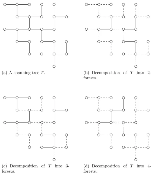
LetK be a positive integer that dividesn−1. Then, the edge set of any spanning tree T ofGcan be partitioned into (n−1)/K acyclic subsets, with K edges each. In other words, T can be decomposed into (n−1)/K forests of K edges each. We will refer to such forests as K-forests. Examples are given in Figure 2.1 for K = 2, 3, and 4.
The basic idea behind the formulation we introduce in this section is to combine K-forests to create spanning trees. To formulate the interaction costs, instead of defin-ing interaction trees for edges, as we did inF1, we define interaction trees forK-forests.
In doing so, even if we relax the requirement that these trees must be equal, the in-teraction trees for the edges in the same K-forest will remain the same. Therefore, the larger the value of K, the closer we are to satisfying the equality constraints. This suggests that this formulation could be stronger than F1.
(a) A spanning tree T. (b) Decomposition of T into 2-forests.
(c) Decomposition of T into 3-forests.
(d) Decomposition of T into 4-forests.
Figure 2.1. Decomposition of a spanning tree intoK-forests, for K= 2, 3 and 4. K-forests are represented by connected components with the same drawing style. In the examples, all K-forests are connected subgraphs of G. Observe however, that this is not always possible in general.
byEK ={H ⊆E :H is K-forest-inducing}the set of allK-forest-inducing subsets of
E and let o=|EK|. Define EK
i ={H ∈EK :i∈H} as the set of the elements of EK
that contain i∈ E. Finally, for all H ∈EK, letX
H =X ∩ {x∈Rm : xi = 1, i∈ H}.
Using similar arguments to those used in the proof of Proposition 2.2 we can show that XH is the convex hull of the incidence vectors of spanning trees containing all edges in
H.
Besides variablesxand yintroduced before, the formulation also employs binary variabless= (sH)H∈EK, such that sH = 1 if and only if H ∈EK is selected to be part
of the solution. To formulate interaction trees, binary variablest= (tHi)H∈EK,i∈E are
used. We denote the row of t indexed by H ∈ EK by t
2.1. Formulations, Linear Programming and Lagrangian Relaxation
Bounds 17
the interaction tree for the K-forest induced by H. QMSTP can be formulated as:
F2 : min
( X
i,j∈E
qijyij : (x,y,s,t)∈P2∩Bm+m
2+o+om
)
,
where polytope P2 is given by:
x∈X, (2.16)
xi =
X
H∈EK i
sH, i∈E, (2.17)
tH ∈(XH ×sH), H ∈EK, (2.18)
yi =
X
H∈EK i
tH, i∈E, (2.19)
yij =yji, i < j ∈E. (2.20)
Constraints (2.16) require thatxdefine a spanning tree ofG. The decomposition of the spanning tree into K-forests is enforced by constraints (2.17). By (2.18), if a K-forest-inducing setH is used in the decomposition, then an interaction tree must be defined for it, otherwise, tH =0. Constraints (2.19) state that, in case edgei appears
in a K-forest that belongs to the solution, then the interaction tree yi for i must be
equal to the interaction tree for that K-forest, otherwise, yi = 0. Finally, by (2.20),
all spanning trees must be equal.
Note that the size of EK is O(mK), which is polynomial in n if K is a constant.
Thus, the size of F2 in relation toF1 is polynomially bounded. Regarding the strength
of F2, when K = 1, formulations F1 and F2 are equivalent. If K = n−1, EK will be
the set of all spanning trees ofG and, consequently,Z(F2) will be the optimal solution
value of QMSTP. For general values of K, we have the following result.
Proposition 2.5. Given a factor K >0of n−1, denote by P2(K)the polytope defined
by (2.16)-(2.20) for this particular value of K. Let Projxy(P2(K)) be the projection of
P2(K) onto the vector space of the variables (x,y) ∈ Rm+m
2
. For two factors K and
L of n−1, L > K, the following holds:
Projxy(P2(L))⊆Projxy(P2(K)).
Proof. Consider a vector (x,y,s,t) ∈ P2(L). We are going to show that there is a
vector (ex,ye,es,et)∈P2(K) such that xe=xand ye=y.
For every H ∈EL define the set EK(H) = {I ∈EK :H ∩I = K}, i.e., EK(H)
c= (L−1)!/((L−K)!(K−1)!) elements of EK(H).
Now, for all I ∈EK let
e
sI =
1 c
X
H∈EL:I∈EK(H)
sH, (2.21)
and
etI =
1 c
X
H∈EL:I∈EK(H)
tH. (2.22)
Thus, from (2.21), for anyi∈E, we have
xi =
X
H∈EL i
sH =
X
H∈EL i
1 c
X
I∈EK(H):i∈I
sH =
X
I∈EK i
1 c
X
H∈EL:I∈EK(H)
sH =
X
I∈EK i
e
sI =xei,
which shows that (2.16) and (2.17) are satisfied inP2(K). From (2.22) we have
yi = X
H∈EL i
tH =
X
H∈EL i
1 c
X
I∈EK(H):i∈I
tH =
X
I∈EK i
1 c
X
H∈EL:I∈EK(H)
tH =
X
I∈EK i
etI =eyi,
which shows that (2.19) and (2.20) are also satisfied inP2(K). Finally, we need to show
that (2.18) is also satisfied. We will only show that, for any I ∈ EK, the cardinality
constraintPi∈EtIi= (n−1)sI is satisfied. The satisfaction of the remaining constraints
can be proved in a similar fashion. Using both (2.21) and (2.22),
X
i∈E
e
tIi =
X
i∈E
1 c
X
H∈EL:I∈EK(H)
tHi =
1 c
X
H∈EL:I∈EK(H)
(n−1)sH = (n−1)seI,
which proves the satisfaction of the desired constraint.
For practical considerations, if K does not divide n −1, we can add artificial vertices to the graph, together with (zero cost) edges to keep the graph connected. Note also that the decomposition of a spanning tree of G intoK-forests might not be unique. However, all that is needed to properly formulate QMSTP is granting that at least one such decomposition exists for any spanning tree. By eliminating redundant possibilities fromEK, we can reduce the number of variables ofF
2 and maybe improve
its LP relaxation bound. The next result shows how that can be accomplished for K ≤4.
Proposition 2.6. Let T be a spanning tree ofG andK be a factor ofn−1. If K = 2,
2.1. Formulations, Linear Programming and Lagrangian Relaxation
Bounds 19
decomposed into K-forests, none of which has more than two connected components.
Proof. Note that, for K = 2, eitherT has edges {i, j}and {j, k} such that iand k are leaves, or iis a leaf and j is not connected to any vertex other than ior k. No matter the case, we remove these two edges to obtain a subgraph of T that is connected and has an even number of edges. The argument is then applied recursively.
For K = 3, remove (1/3)(n − 1) edges {i, j} of T, one at a time, under the condition that i is a leaf. The remaining subgraph has (2/3)(n − 1) edges and is connected; apply the procedure for K = 2 to this subgraph. For each resulting set of two edges, add one of the edges that were previously removed.
ForK = 4, apply the procedure forK = 2, group the resulting pairs of adjacent edges into sets of four edges.
Even in the light of Proposition 2.6, computing Z(F2) by explicitly solving LPs
is impractical, due to the large number of variables and constraints that compose F2.
Recall that formulation F2 was developed with the relaxation of constraints (2.20) in
mind. We will now investigate the relaxation and the dualization of those constraints in a Lagrangian fashion. To that aim, consider again that unconstrained multipliers θ = (θij)i<j∈E, defined as before, are assigned to (2.20). Such a relaxation strategy
leads to the following Lagrangian subproblem:
F2′(θ) : L′2(θ) = min
( X
i,j∈E
qij′ yij : (x,y,s,t)∈P2′ ∩Bm+m
2+o+om
)
,
where P′
2 is obtained by relaxing (2.20) in P2, i.e., P2′ is represented by (2.16)-(2.19).
Lagrangian modified costs are defined as q′ij = qij +θij for all i6= j ∈E and qii′ =qii
for all i∈E.
Observe that, by (2.19), the objective function of F′
2 can be written as:
X
i,j∈E
qij′ yij =
X
i,j∈E
X
H∈EK i
q′ijtHj =
X
H∈EK
X
i∈H
X
j∈E
qij′ tHj.
Therefore, using the fact that in F′
2 the choice of the spanning tree tH depends
only on sH, it can be concluded that in an optimal solution (x,y,s,t) for F2′(θ), for
some particular choice of multipliers θ, if sH = 1, tH will be the incidence vector of a
spanning tree that minimizes:
qH = min
( X
i∈H
X
j∈E
q′ijtHj :tH ∈XH ∩Bm
)
Thus, problemF′
2 can be solved with the resolution of
q0 = min
X
H∈EK
qHsH :x∈X;xi =
X
H∈EK i
sH,∀i∈E; (x,s)∈Bm+o
, (2.24)
followed by the appropriate adjustment ofy and t. This process is summarized in the following algorithm.
Algorithm 2:
Input: A QMSTP instance given by G = (V, E) and Q ∈ Rm+2. A factor K of
n−1. A set of Lagrangian multipliers θ ∈Rm(m2−1).
Output: A Solution (x,y,s,t) forF2′(θ).
1. For every H ∈EK, solve (2.23) and denote byet
H its solution vector.
2. Solve problem (2.24) to obtain a solution (ex,es).
3. Obtain a solution (x,y,s,t) of costL′2(θ) = q0 forF2′(θ) by makingx=ex,s=es,
tH =sHetH for all H ∈EK, and yi =
P
H∈EK
i tH for all i∈E.
While Algorithm 2 actually solvesF2′, the problem is in fact NP-Hard forK ≥3. Consequently, it is unlikely that one can come up with an efficient algorithm to solve step 2, in particular.
Proposition 2.7. Problem F′
2 is NP-Hard for K ≥3
Proof. Deciding whether a (K + 1)-uniform hypergraph has a spanning tree is NP-Complete for K ≥3. For K = 2, while the decision problem can be solved in polyno-mial time, the minimization problem is still an open problem [43]. The idea of the proof is to reduce the decision problem to F′
2, defined over forests of size K. The detailed
proof is presented in Section B.1 of the Appendix.
Given the complexity of solvingF′
2, we study two possible alternative approaches
to derive lower bounds from relaxations of that formulation.
2.1.2.1 First Approach - Selecting Edge-disjoint K-Forests
Consider the subtour elimination constraints (SECs) (2.2). For integer solutions ofF2,
2.1. Formulations, Linear Programming and Lagrangian Relaxation
Bounds 21
that, observe that
yij =yji ≤xj, i, j ∈E,
and asyi defines a spanning tree,xalso defines a spanning tree. Moreover, by further
relaxing and dualizing (2.2) in F′
2, the resulting problem consists of selecting (n −
1)/K non-overlapping K-forests, i.e., their union do not need to be acyclic, while also selecting independent interaction trees for each of them. This problem is easy to solve for a particular value of K. Such a relaxation is studied in what follows.
Let µ = (µS)S⊂V,|S|≥2, be a set of non-negative multipliers associated to
con-straints (2.2). As before, let θ = (θij)i<j∈E be unconstrained multipliers associated
to (2.20). After the two sets of constraints are relaxed and dualized, the following Lagrangian subproblem results:
F2′′(θ, µ) :L′′2(θ, µ) = C+ min
( X
i,j∈E
qij′ yij : (x,y,s,t)∈P2′′∩Bm+m
2+o+om
)
,
where P′′
2 is obtained by relaxing (2.20) and (2.2) in P2, i.e., P2′′ is defined by (2.1),
(2.3), (2.17)-(2.19). Lagrangian costs q′
ij are defined as qij′ = qij +θij if i 6= j ∈ E,
q′
ii =qii+PS⊂V,|S|≥2,i∈E(S)µS,i∈E, and C =−
P
S⊂V,|S|≥2µS(|S| −1).
The associated Lagrangian dual is:
DF2 : L′′∗2 = max
n
L2′′(θ, µ) : (θ, µ)∈Rm(m2−1) ×R|{S⊂V,|S|≥2}|
+
o
.
Let (x,y,s,t) be an optimal solution for F′′
2(θ, µ) for some particular choice of
Lagrangian multipliers (θ, µ). If sH = 1, then (x,y,s,t) can be so that tH is the
incidence vector of the spanning tree that minimizes (2.23). Also, after the relaxation of (2.2), variables x can be eliminated from the formulation. This way, F′′
2(θ, µ) can
be solved with the resolution of
q0 =C+ min
X
H∈EK
qHsH :
X
H∈EK i
sH ≤1,∀i∈E;
X
H∈EK
sH =
n−1
K ;s∈B
o
, (2.25)
and the appropriate adjustment of x, y, and t. Problem (2.25) asks for the optimal selection of (n−1)/K K-forests ofG such that no edge iappears in more than one of them. In other words, (2.25) is a set packing problem with an additional cardinality constraint. This problem can be efficiently solved forK = 2 but is NP-Hard forK ≥3.
Proposition 2.8. Problem F′′
Proof. We provide a polynomial reduction from the problem of deciding whether aK -uniform hypergraph has a perfect matching. That problem is NP-Complete forK ≥3. Details of the reduction are given in Section B.2 of the Appendix.
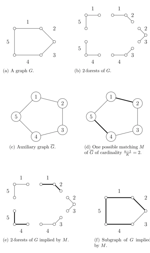
If K = 2, problem (2.25) requires the optimal selection of (n − 1)/2 non-overlapping 2-forests. In other words, one has to find a minimum cost matching of cardinality (n−1)/2, in an auxiliary graphG= (V , E), defined with vertex setV =E and edge set E = EK. An example is given in Figure 2.2. Finding a matching with
fixed cardinality of a graph can be done in polynomial time, an algorithm is given in [41]. That algorithm is used as the basis of Algorithm 3 below, for the resolution of (2.25).
Algorithm 3:
Input: QMSTP instance given by G = (V, E) and Q ∈ Rm2
+ . Set of costs qH for
eachH ∈EK, K = 2.
Output: Solution (x,s) for (2.25).
1. Define an auxiliary graph G= (V , E), where V =E and E =EK.
2. LetU be a set of m−(n−1) auxiliary vertices. Set V =V ∪U.
3. LetJ ={{u, v}:u∈U, v ∈V} and qH = 0 for all H ∈J. Set E =E∪J.
4. Find a minimum cost perfect matching of G, let s be its incidence vector. For all i ∈ E, if there is an H ∈ EK
i such that sH = 1, set xi = 1. Otherwise, set
xi = 0.
2.1. Formulations, Linear Programming and Lagrangian Relaxation
Bounds 23
1
2
3 4
5
(a) A graphG.
1
5
5
4
1 2
3 2
3 4
(b) 2-forests of G.
1
2
3 4
5
(c) Auxiliary graphG.
1
2
3 4
5
(d) One possible matchingM
ofGof cardinality n−1 K = 2.
1
5
5
4
1 2
3 2
3 4
(e) 2-forests ofGimplied byM.
1
2
3 4
5
(f) Subgraph of G implied byM.
Figure 2.2. Using an auxiliary graph G in order to find a set of (n−1)/K
In order to solve F′′
2(θ, µ) for K = 2, we can proceed by computing the costs
(2.23), followed by the resolution of (2.25) by Algorithm 3. Algorithm 4 summarizes the main steps.
Algorithm 4:
Input: QMSTP instance given by G = (V, E) and Q ∈ Rm+2. Set of Lagrangian
multipliers (θ, µ)∈Rm(m2−1) ×R|{+S⊂V,|S|≥2}| .
Output: Solution (x,y,s,t) for F2′′(θ, µ) for K = 2. 1. Solve problem (2.23) for eachH ∈EK and letet
H be the minimizing vector.
2. Solve (2.25) by Algorithm 3. Let (ex,es) denote a solution.
3. Obtain a solution (x,y,s,t) of cost L′′2(θ, µ) =q0 for F2′′(θ, µ) by letting s =es
and x=xe. Let tH =sHetH for all H ∈EK, and yi =
P
H∈EK
i ti for all i∈E.
The first step of Algorithm 4 can be implemented to run in O(omlogn) = O(m3logn) time complexity. Algorithm 3 can be implemented to run inO(|V|2|E|) =
O(m4) [21]. This gives the complexity of step 2, which determines the overall worst case time complexity of Algorithm 4.
As a result of the discussion above, the solutions for the Lagrangian subproblem F′′
2(θ, µ) implicitly satisfy all valid inequalities for the matching polytope. Since the
blossom inequalities [15] (facet defining inequalities for the matching polytope) are missing fromF′′
2, the Lagrangian dual bound provided by DF2 might well be stronger
thanZ(F2).
Proposition 2.9. L′′∗
2 ≥Z(F2).
The evaluation of L′′∗2 requires finding optimal multipliers for an exponential number of constraints (2.2). One of the known algorithmic alternatives to deal with exponentially many inequalities candidates to Lagrangian dualization is the relax-and-cut approach [30]. Due to the already excessive (though polynomial in n, m) number of other dualized constraints, the benefits of implementing a relax-and-cut algorithm for the evaluation ofL′′∗
2 are quite small: in practice, small lower bound improvements
are obtained at a substantial increase of CPU time. Thus, we consider an algorithm for computing QMSTP lower bounds based onDF2 whereµ=0,θ is adjusted by the
2.1. Formulations, Linear Programming and Lagrangian Relaxation
Bounds 25
algorithm is denoted Lag2. A BB algorithm based onLag2 is presented in Section 2.2.
We report computational results for Lag2 in Section 2.3.
2.1.2.2 Second Approach - Variable Splitting
In this section, we present a reformulation ofF2that preserves its LP relaxation bounds.
The interesting aspect of this reformulation is that a Lagrangian relaxation scheme, with easy to solve subproblems, can be developed to evaluate its LP lower bounds. On the downside, the Lagrangian relaxation scheme needs to deal with a very large number of dualized constraints.
Consider the replacement of each variable sH, for all H ∈EK, by K new binary
variables siH, one for each i ∈ H, so that now we have s = (siH)i∈E,H∈EK i . We
denote by si = (siH)H∈EK
i the row of s indexed by i ∈ E. Likewise, consider the
replacement of each vector tH byK new binary vectorstiH, one for eachi∈H. Then,
t= (tiHj)i,j∈E,H∈EK
i and we denote by ti = (tiH)H∈EiK the entries of t with first index
i ∈ E, and by tiH = (tiHj)j∈E the row of ti indexed by H ∈ EK. QMSTP can be
formulated as:
F3 : min
( X
i,j∈E
qijyij : (x,y,s,t)∈P3∩Bm+m
2+Ko+Kom
)
, (2.26)
where P3 denotes the polytope given by:
x∈X, (2.27)
xi =
X
H∈EK i
siH, i∈E, (2.28)
yi =
X
H∈EK i
tiH, i∈E, (2.29)
tiH ∈(XH ×siH), i∈E, H ∈EiK, (2.30)
yij =yji, i < j ∈E, (2.31)
siH =sjH, i < j ∈E, H ∈EiK∩EjK. (2.32)
Later, we will show that the relaxation of constraints (2.31) and (2.32) results in a problem that is easy to solve for any factor K, what allows us to develop a tractable lower bounding procedure based onF3. Before discussing that, observe that constraints
of type (2.32) were not imposed for t, what implies that Z(F3) may be weaker than
Z(F2). This can be overcome by conveniently rewriting the objective function of F3.
(2.32),
X
k∈H
tkHj =K. (2.33)
Using (2.29) and (2.33), the objective function in (2.26) can be rewritten as:
X
i,j∈E
qijyij =
X
i∈E
X
H∈EK i
X
j∈E
qijtiHj =
X
i∈E
X
H∈EK i
X
j∈E
X
k∈H
1
KqijtkHjtiHj.
Note thattiHjtkHj =tiHj =tkHj for any i, j, k∈E and H ∈EiK ∩EkK. Therefore
X
i∈E
X
H∈EK i
X
j∈E
X
k∈H
1
KqijtkHjtiHj =
X
i∈E
X
H∈EK i
X
j∈E
X
k∈H
1
KqijtkHj
=X
i∈E
X
H∈EK i
X
j∈E
X
k∈H
1
KqkjtiHj (2.34)
In other words, (2.34) states that the cost of the tree defined by tiH, for some i ∈ E
andH ∈EK
i , depends equally on all the edges in H and their interaction costs. In the
remainder of this section, we assume that the objective in (2.26) is rewritten according to (2.34). Bearing that in mind, we have the following result.
Proposition 2.10. Z(F2) =Z(F3).
Proof. We make use of an argument based on the application of Lagrangian relaxation to the LP relaxations ofF2 and F3. We dualize constraints (2.31) with unconstrained
Lagrangian multipliersθ = (θij)i<j∈E, defined as before. This gives the the Lagrangian
subproblem
F3′(θ) :L′3(θ) = min
( X
i∈E
X
H∈EK i
X
j∈E
X
k∈H
1 Kq
′
kjtiHj : (x,y,s,t)∈P3′ ∩Bm+m
2+Ko+Kom
)
,
where P′
3 is obtained by relaxing (2.31) in P3, i.e., P3′ is defined by (2.27)-(2.30) and
(2.32). Lagrangian modified costs are defined as q′ij = qij +θij for i 6= j ∈ E and
qii′ =qii for i∈E.
We now show that for any θ ∈ Rm(m2−1), Z(F′
3(θ)) = Z(F2′(θ)), which proves the
claim.
Given a feasible solution (x,y,s,t) for the LP relaxation ofF′
2(θ), letting ex=x,
e
y=y,esiH =sH andetiH =tH for alli∈H and H ∈EiK, we obtain a feasible solution
(xe,ey,es,et), with the same objective value for the LP relaxation of F′
3(θ).
Conversely, by (2.34), given a solution for the linear relaxation of F′
3(θ), there is
2.1. Formulations, Linear Programming and Lagrangian Relaxation
Bounds 27
for any i, j ∈ E and H ∈ EK
i ∩EjK. Letting x= ex, y =ye, sH =esiH, and tH =etiH,
for all H∈EK and somei∈H, we obtain a feasible solution (x,y,s,t) with the same
objective value for the LP relaxation of F′
2(θ).
When constraints (2.31) and (2.32) are relaxed in F3, we obtain a problem
that is easy to solve for any value of K. Consider again unconstrained dual mul-tipliers θ = (θij)i<j∈E attached to (2.31). Define unconstrained multipliers π =
(πijH)i<j∈E,H∈EK
i ∩EjK, attached to (2.32). Assume πiiH = 0 for all i ∈ E, and
πijH = −πjiH, for all pairs i > j ∈ E and H ∈ EiK ∩EjK. Then, we obtain the
Lagrangian subproblem:
F3′′(θ, π) : L′′3(θ, π) = min
( X
i∈E
X
H∈EK i
X
j∈H
(πijHsiH +
X
k∈E
1 Kq
′
jktiHk)
: (x,y,s,t)∈P3′′∩Bm+m2+Ko+Kom
)
,
where P′′
3 is obtained by relaxing (2.31) and (2.32) inP3, i.e., P3′′ is defined by
(2.27)-(2.30). The modified costs are defined as qij′ =qij +θij for i6=j ∈E and qii′ =qii for
i∈E. The associated Lagrangian dual is:
DF3 : L′′∗3 = max
n
L′′3(θ, π) : (θ, π)∈Rm(m2−1)+
oK(K−1) 2
o
.
To see how F′′
3(θ, π) can be solved for any choice of multipliers (θ, π) ∈
Rm(m2−1)+
oK(K−1)
2 , consider an optimal solution (x,y,s,t). We see that if xi = 1 for some i ∈ E, and siH = 1 for some H ∈ EiK, then tiH is the incidence vector of the
spanning tree that minimizes
qiH = 1
K min
( X
j∈H
X
k∈E
qjk′ tiHk :tiH ∈XH ∩Bm
)
. (2.35)
Therefore, if xi = 1, i∈E, we have siH = 1 for the element of HiK that minimizes
qi = min
(
qiH+
X
j∈H
πijH :H ∈EiK
)
. (2.36)
Thus, F3′′ can be solved by solving
q0 = min
( X
i∈E
qixi :x∈X∩Bm
)
followed by the appropriate adjustment of y, s, and t. The following algorithm sum-marizes the procedure.
Algorithm 5:
Input: QMSTP instance given by G = (V, E) and Q ∈ Rm+2. Set of Lagrangian
multipliers (θ, π)∈Rm(m2−1)+
oK(K−1) 2 .
Output: Solution (x,y,s,t) for F′′
3(θ, π).
1. Solve (2.35) and obtainqiH for eachi∈E and H ∈EK
i . Denote the minimizing
vector byetiH. Observe that (2.35) needs to be solved only once for eachH ∈EK,
i.e., find qiH for some i∈H and let qjH =qiH andetjH =etiH for all j 6=i∈H.
2. Solve (2.36) for eachi∈E to obtain qi. Let esiH = 1 for the minimizing element
H ∈EK
i and esiI = 0 for the remaining I 6=H ∈EiK.
3. Solve the minimum spanning tree problem in (2.37) and denote the minimizing vector by ex.
4. Obtain a solution vector (x,y,s,t) of cost q0 =L′′
3(θ, π) for F3′′(θ, π) by letting
x = ex, siH = xeiseiH and tiH = siHetiH for all i ∈ E and H ∈ EiK, and yi =
P
H∈EK
i tiH for all i∈E.
Steps 1 and 2 can be implemented to run in O(omlogn) = O(mK+1logn) and
O(Ko) =O(KmK) time, respectively. AnO(mlogn) implementation can be given for
Step 3. Thus, the overall time complexity of the algorithm is defined by Step 1. In order to evaluate the strength of DF3, we first present the following result.
Proposition 2.11. P3′′ is an integral polytope.
Proof. The proof is quite similar to the proof of Proposition 2.4 and is presented in Section B.3 of the Appendix.
By Propositions 2.10 and 2.11, we obtain
Corollary 2.3. L′′∗
3 =Z(F2) = Z(F3).
To solve DF3, we have to deal with the large number of dualized constraints,
O(KmK) in general. We faced convergence difficulties when applying subgradient
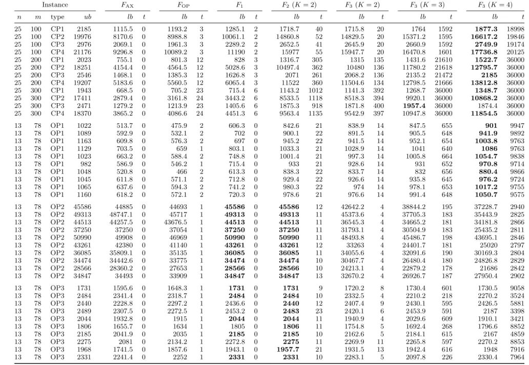


![Table D.1. QMSTP branch-and-bound results. Instances of Cordone and Passeri [13].](https://thumb-eu.123doks.com/thumbv2/123dok_br/15178609.17848/100.1262.243.1038.124.723/table-qmstp-branch-bound-results-instances-cordone-passeri.webp)
![Table D.2. QMSTP branch-and-bound results. Instances of ¨ Oncan and Punnen [35], type 1.](https://thumb-eu.123doks.com/thumbv2/123dok_br/15178609.17848/101.1262.276.970.159.682/table-qmstp-branch-bound-results-instances-oncan-punnen.webp)
![Table D.3. QMSTP branch-and-bound results. Instances of ¨ Oncan and Punnen [35], type 1.](https://thumb-eu.123doks.com/thumbv2/123dok_br/15178609.17848/102.1262.282.1008.154.684/table-qmstp-branch-bound-results-instances-oncan-punnen.webp)
