Abstract: This work presents an algorithm for solving exactly a scheduling problem with identical

Solving a Multiprocessor Problem by Column Generation

and Branch-and-price

António J. S. T. Duarte*, J. M. Valério de Carvalho**

*Polytechnic Institute of Bragança, Bragança, Portugal (e-mail: aduarte@ipb.pt) **University of Minho, Braga, Portugal (e-mail: vc@dps.uminho.pt)

Abstract: This work presents an algorithm for solving exactly a scheduling problem with identical parallel machines and malleable tasks, subject to arbitrary release dates and due dates. The objective is to minimize a function of late work and setup costs. A task is malleable if we can freely change the set of machines assigned to its processing over the time horizon. We present an integer programming model, a Dantzig-Wolfe decomposition reformulation and its solution by column generation. We also developed an equivalent network flow model, used for the branching phase. Finally, we carried out extensive computational tests to verify the algorithm’s efficiency and to determine the model’s sensitivity to instance size parameters: the number of machines, the number of tasks and the size of the planning horizon.

1. PROBLEM DEFINITION

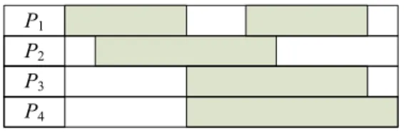
Given a set of tasks (T1, T2, …, Tn) and a set of machines (P1, P2, …, Pm), the objective is to find a feasible schedule that minimizes a function of the number of setups and the amount of late work. The tasks allow for preemptions, multiprocessing and are malleable (Blazewicz et al., 2004). This last property means that we can freely change the set of machines processing a given task over the time horizon, as shown in the next machine schedule:

P1

P2

P3

P4

Fig. 1. Scheduling of a malleable task

The task (in shadow) is scheduled in four machines, and the number of machines assigned to the task may vary arbitrarily over time.

1.1 Machines

The problem considers a set of m identical machines,

{

1, 2, , m

}

P= P P  P . Each machine can only process one task at a time and they can be preempted at arbitrary moments. Because of computational complexity issues, in our models we will only allow preemptions at integer time units. This can be done without loss of generality, because the time unit can be freely chosen, according to the problem requirements and the available computational resources.

1.2 Tasks

For the definition of the task environment, we use a set of n tasks, T =

{

T T1, 2,,Tn

}

. Each task has a processing time (p_j), a release date (r_j), a due date (dj) and a weight for the

calculation of late work cost (wj).

Although the values of pj , rj and dj can be any

nonnegative numbers, for consistency with the machine environment, we limit these values to nonnegative integers.

A machine schedule can be seen as a sequence of unit fragments of different tasks. If two consecutive fragments belong to the same task there is no setup cost, otherwise, a setup cost is incurred. Although a setup requires, among other resources, a certain amount of time, in our models, we assume that setup times are very short when compared to production runs. Therefore, we will only minimize the total number of setups.

1.3 Objective Function

Let c_k be the cost of schedule k (a single machine schedule). We define ck in the following way:

k k k

c =l +s ₍₁₎

In the previous equation l_k is the cost incurred because of late work in schedule k and sk is the number of setups in the schedule. The value of lk is calculated according to the late work in the schedule and to the values of the w_j constants. The values for wj must be chosen wisely because there is an implicit trade-off with the setup costs. Also, the model for calculation of l_k can be subject of discussion.

distant from the task due date. The total late work penalty for a given machine schedule can be computed as follows:

(

)

1 jk

n

k j l j

j l L

l w C d

= ∈

=

 

− ₍₂₎

In the above equation, Ljk represents the set of late fragments

belonging to task Tj present at schedule k and Cl is the completion time for each one of those fragments. This function can be replaced with any function compatible with the subproblem algorithm, which will be presented later on this paper.

Note that the total cost of a given schedule is the sum of costs of every machine and that it is possible to calculate the contribution of each machine schedule to the total cost without knowing the schedules of the other machines.

2. PROBLEM FORMULATION

2.1 A Simple Network Flow Model

We will show below that the problem presented in the previous section can be modeled as a network flow problem and solved with a suitable algorithm. Although the network flow model always provides valid solutions for the problem, it is insensitive to setup costs and an optimal solution cannot be directly obtained from it. However, the solutions can be improved by heuristics and used as upper bounds in the branch-and-price algorithm.

Essentially, the network flow model is a transportation model similar to Horn’s model (Horn, 1973). The problem will have j origins (one per task) with supplies equal to the processing times, p_j. Let us call each origin Tj. On the other hand,

each possible time slot in the schedule will become a destination with demand equal to the number of available machines, m. We will call each destination It and it refers to the scheduling period

[

t−1,t

]

. The index t can vary between 1 and tmax (which defines the time horizon for the problem). In order to balance the problem, an additional origin must be set to supply the idle time in the schedule. Let that origin be

L

T . Its supply is:

1 n

max j

j

mt p

=

−



(3)

This value cannot be negative. In that event there would be no feasible solutions, because the processing times would exceed the available capacity.

The following figure represents the proposed model:

1 T

2 I



max

t I 2

T

L T



1 I

jt c

Fig. 2. Network flow model

Note that arc

(

T I_j, _t

)

will only exist if rj≥ −t 1. Otherwise, the task is not available for processing at t−1. The value cjt refers to the cost of each arc and is computed in the following way:

(

)

0,

, j jt

j j j

d t c

w t d d t

≥



=

− <

 (4)

This computation must agree with the cost function defined in section 1.3 and assures that late work costs will be minimized.

Preposition 1: If all tasks have unit processing times, the solution obtained from the proposed network flow model is optimal.

Proof: If all processing times are unitary, all tasks are scheduled in exactly one scheduling slot, incurring in one setup. The total number of setups will be equal to the number of tasks and it will be optimal.

In the next section we discuss an algorithm to transform a network flow model solution into a valid scheduling solution with minimal number of setups.

2.2 Obtaining a Valid Scheduling Solution

Obtaining a valid scheduling solution to our problem from a network flow solution is trivial. In this section we propose an algorithm that not only achieves a valid solution but also minimizes the number of setups for the given network flow solution.

Let fjt be the flow from Tj to It in a given network flow solution. The network flow solution will be completely defined by the following flow matrix, F:

11 12 1

21 22 2

1 2

max

max

max

t t

n n nt

f f f

f f f

F

f f f

 

 

 

=_{ }

 

 

 





   



(5)

Because all values for demand and supply are integers, it is guaranteed that all flow values are also integers. It can easily

be shown that, for every time slot, 1 n

jt j

f m

=

≤



. In fact, this sum is the number of machines in use for each time slot. Then, for t=1 the number of incurred setups is equal to

1 1 n

j j

f =



.

On subsequent time slots, for any given machine, setups are not necessary if the scheduled task is the same task scheduled in the previous time slot. In general, at time t, we can avoid, at most, a number of setups equal to

(

1

)

1

min , n

jt jt j

f f ₊ =



. The

To obtain a solution we first schedule the flows for t=1 and proceed chronologically until t=tmax. For each time slot the

t

F vector is decomposed into two vectors: the vector of flows that can be scheduled without setups, C

t

F , and the vector of flows that need setups, FtD. Obviously,

C D

t t t

F =F +F . The two vectors can be calculated as follows:

(

1

)

min , C

jt jt jt

f = f ₋ f ₍₆₎

D C

jt jt jt

f = f − f

(7) For the initialization, we must admit fj0 =0 for all tasks. This will force 1 0

C j

f = for all tasks and a setup for each machine used at time t=1.

At t=1 the choice of machines to schedule flows is irrelevant (a setup will be needed for each used slot). In subsequent periods the flows in vector C

t

F must be scheduled first in machines that have the same task on the previous period. The flows in D

t

F are always scheduled last and the choice of machine is irrelevant.

This algorithm is polynomial with respect to n, m and t_max. Preposition 2: Applying the algorithm to a given set of flows results in a minimal number of setups for that set of flows.

Proof: For t=1 a setup is unavoidable for each used machine. For subsequent periods and for each task, if

1 jt jt

f ≤ f ₋ no setups are needed for that task. In that case C

jt jt

f = f and no setup will be incurred. If f_jt > f_jt−1, at least 1

jt jt

f − f _{− must be incurred. Now,} D ₁

jt jt jt

f = f − f _{− and only} the minimal number of setups is incurred.

In the following section we will present the integer linear programming model used to obtain the optimal solution to the problem.

2.3 Integer Programming Model

As the network flow model presented on the previous sections does not provide an optimal solution to the problem, we developed an integer programming approach to solve the problem. In this section we present the developed model.

The proposed formulation is based on time indexed variables. This kind of variables was first used to solve scheduling problems by Sousa et al. (1992). In this context, we use the binary variables xijt which takes the value 1 if task j is scheduled on machine i at time slot t, which represents the period

[

t−1,t

]

. Otherwise, these variables will take the value 0.

To account for the number of setups we must also introduce a set of binary variables, yijt . If setting xijt =1 a setup is

incurred, and the corresponding variable, y_ijt, must take the

value 1. If x_ijt=0 or no setup is incurred, the corresponding y variable takes the value 0.

The complete ILP model is as follows:

(

)

1 1 1 1 1 1

max max

j

t t

m n m n

ijt j j ijt

i j t i j t d

min y w t d x

= = = = = = +

+ −



 

₍₈₎

1 1

. . ,

max

t m

ijt j i t

s t x p j

= =

= ∀



(9)

1

1, , n

ijt j

x i t

=

≤ ∀ ∀



₍₁₀₎

1 1, , ij ij

y =x ∀ ∀i j ₍₁₁₎

{

}

1, , , 2, 3, ,

ijt ijt ijt max

y ≥x −x ₋ ∀ ∀ ∀ ∈i j t  t

(12) 0,1, , ,

ijt

x = ∀ ∀ ∀i j t ₍₁₃₎

0,1, , ,

ijt

y = ∀ ∀ ∀i j t

(14) The objective function (8) follows from section 1.3, in terms

of the x and y variable meanings. The first term accounts for the number of setups and thus, the setup costs. The second term accounts for the late work costs.

Constraints (9) ensure that each task is scheduled in p_j time slots and, therefore, the processing times are met. The next set of constraints (10) ensures that, at most, one task is scheduled at each time slot. Note that they also assure that no more that m machines are used in each time unit.

Constraints (11) ensure that a setup is accounted for any task scheduled at time slot 1. Constraints (12) guarantee that, in any machine and in every time slot, if the scheduled task is different from the task scheduled in the previous time slot the appropriate y variable takes the value 1.

This problem is not amenable for solution with a commercial optimization package for two reasons: first, the number of variables and constraints rises rapidly with the number of machines, the number of tasks or the planning horizon size; second, the problem is very symmetric, because the same scheduling solution can be implemented with different machine indexes.

For those reasons we implemented a column generation approach to solve the problem that is presented in the next section.

3. COLUMN GENERATION

In this section we start by presenting a Dantzig-Wolfe decomposition of the model and a dynamic programming algorithm for solving the resulting subproblem. Later in the section we propose a branching scheme and we discuss the corresponding implications on the subproblem algorithm.

3.1 Dantzig-Wolfe Decomposition

Consider the mathematical model presented in section 2.3. For simplicity, the following transformations will be performed:

i

i

C : a vector of all objective function coefficients referring to processor i;

i

A : a matrix with j rows containing all the coefficients referring to machine i for the processing times constraints;

p: the vector of processing times;

i

P: a polyhedron defined by all the constraints (except the processing times constraints) that refer to machine i.

Using these later definitions, the mathematical model can be rewritten as follows:

1 1 . . , m T i i i m i i i i i min s t P i = = = ∈ ∀





C Z

A Z p

Z

(15)

The set of constraints with a block angular structure was decomposed, leaving the processing times constraints in the master problem and defining a subproblem for each P_i constraint.

3.1.1 The Master Problem

Because P_i is a convex region, any point of that region can be represented as a convex combination of extreme points. Let Ki be the set of extreme points for machine i and let Pki

represent an element of that set. This can be translated to the following equality:

, 1, 0,

i i i i

i i i i

i k k k k i

k K k K

Pλ λ λ k

∈ ∈

=





= ≥ ∀

Z

(16)

After variable substitution the master problem is as follows:

(

)

(

)

1 1 . . 1, i i i i i i i i i i i m T

i k k

i k K m

i k k i k K

k k K

min P

s t P

i λ λ λ = ∈ = ∈ ∈ = = ∀

 

 



C A p (17)

Because, in our problem, the processors are identical, the reference to the specific processor can be removed and the convexity constraints can be replaced by their sum:

(

)

(

)

. . T k k k K k k k K k k K min P

s t P

m λ λ λ ∈ ∈ ∈ = =







C A p (18)

For simplicity, let xk =λk ,

T k k

c =C P and ajk be the elements of AP_k. After the necessary substitutions the master problem can be written as follows:

. . , k k k K

jk k j k K

k k K min c x

s t a x p j

x m ∈ ∈ ∈ = ∀ =







(19)

In this last model a variable can be seen as a schedule for one processor, where c_k is the contribution of that schedule to the global cost and ajk is the amount of processing done for task j in that schedule. The collection of all individual machine schedules present in the optimal solution will make up the global schedule. Based on this interpretation the following conclusion can be drawn.

Preposition 3: For a solution to be integral, it is sufficient that all x_k variables have integer values.

Proof: The value of each variable is the number of processors executing the corresponding schedule. Thus, if all variables have integer values the solution can be translated to a valid operational plan.

However, as we will show later, this is not a necessary condition to get a valid solution.

In order to generate new individual machine schedules to include in the master problem, each schedule cost must be determined without knowing in advance the global schedule. As remarked in section 1.3, our objective function complies with this requirement.

It is known that, whenever possible, replacing equality constraints with inequalities leads to better computational performance because the additional restriction of the dual solution space (Desaulniers et al., 2002). As shown next, all the equalities in our master problem can be replaced with inequalities.

Preposition 4: All the constraints in the form jk k j k K

a x p

∈

=



can be replaced with constraints in the form jk k j

k K

a x p

∈

≥



.

Proof: If a task processing time is exceeded the extra processing can always be removed from the end of the schedule without additional setups or late work.

Preposition 5: The constraint k k K

x m

∈

=



can be replaced by the constraint k

k K

x m

∈

≤



.

Proof: If allowed by the processing times, machines can be left idle.

Making these two transformations, the resulting master problem will be:

. . , k k k K

jk k j k K

k k K min c x

3.1.2 The Subproblem

Let π_j (for j=1, 2,,n ) be the set of dual variables associated with the first n constraints of the master problem and let π_M be the dual variable associated with the last constraint. To find the column with the maximum reduced cost for the master problem, the following subproblem is solved:

(

)

{

}

1 1 1 1 1 1

1

1 1

1

. . 1,

,

, , 2, 3, ,

0,1, , 0,1, ,

max max max

j

t t t

n n n

j jt M jt j j jt

j t j t j t d

n jt j

j j

jt jt jt max

jt jt

max x y w t d x

s t x t

y x j

y x x j t t

x j t

y j t

π π

= = = = = = +

=

−

+ − − −

≤ ∀

= ∀

≥ − ∀ ∀ ∈

= ∀ ∀

= ∀ ∀





 





(21)

Note that this problem is still hard to solve with a general ILP software package. However it has a special structure that allows the development of a specialized algorithm presented in the next section.

In the objective function, πj can be seen as a prize for including each unit of task j processing in the schedule. The constant πM (negative) is the penalty for using the processor pool (independently of the schedule). The rest of the objective function, as before, deals with the penalties incurred for setups and late work.

In the next section a dynamic programming algorithm that takes advantage of the subproblem’s structure is presented.

3.2 Dynamic Programming Algorithm for the Subproblem In order to identify new attractive columns to include in the master problem we developed a dynamic programming algorithm that takes advantage of the subproblem special structure.

The developed algorithm has t_max+1 stages, corresponding to each integral time instant from 0 to t_max, and n+1 states, representing the last scheduled task (one of the n tasks or none). Note that, because of the release dates, not all states are available at every stage.

Let F jt

( )

be the objective function value for state j and

stage t. For simplicity assume that at time t=0 (stage 0) the machine is not set to any task, i.e., the machine is at state 0. We can start up the dynamic programming algorithm by setting the initial objective function value:

( )

0 0 M

F =π ₍₂₂₎

This means that, if no task is scheduled, the reduced cost of the new column will be π_M . For any stage, the objective function value can be calculated recursively by the following expression:

( )

max

(

1

( )

)

t t j tj lj

F j = F− l +π −w −p _{, (23)}

where t=1, 2,,t_max and j=

{

0, :j r_j <t

}

and

{

0, : _j 1

}

l= j r < −t . We must also define π0 =0 and the

values of w_tj and p_lj:

(

)

0, 0

, 0

j tj

j j j

j or t d w

w t d j and t d

= ≤



=

− > >

 (24)

0, 0 1, 0 lj

j or l j p

j and l j

= =



=

> ≠

 ₍₂₅₎

These last expressions will account the setup costs (25) and the late work costs (24), as explained.

The iterative solution of the master problem (to obtain a dual vector for the subproblem) and of the subproblem (to obtain new columns for the master problem) until there are no more attractive columns will lead to an optimal solution to the linear relaxation of the master problem. Usually, this optimal solution will not obey the integral requirements of the master problem. To get an optimal integral solution we developed the branching scheme presented in the following section.

3.3 Branching Scheme

Branching on the restricted master problem variables is not a good choice, because it may lead to column regeneration (Barnhart, 1998). We do not branch on those variables, but rather on the variables of the network flow model.

Previously we defined fjt as the network flow model

variable representing the flow in arc

(

T I_j, _t

)

. This variable represents the number of processors allotted to task j at time slot t. A relation between the flow variables and the restricted master problem can be established by the following expression:

jt jtk k

k K

f δ x

∈

=



(26)

The δjtk coefficients are equal to 1 if, in processor schedule

k, the j task is scheduled at time slot t, and are equal to 0 otherwise. These coefficients must be determined at column generation because they cannot be calculated based on the master problem technological coefficients.

Preposition 6: A solution is integer iff all fjt are integer.

Proof: The condition is sufficient because, on any integral set of flows, we can apply the algorithm described in section 2.2 to obtain a valid scheduling solution. The condition is necessary because any value of fjt represents the number of

machines allotted to task j at time slot t, which must be integer.

If a solution has non-integer flows, one of those flows must be chosen for branching. Because this choice may be computationally relevant, a method for choosing the flows to branch on may be needed. Let us denote the value of the non-integral flow to branch on by *

jt

f . The current problem (corresponding to a branch tree node) will originate two child problems with a mutually exclusive set of solutions: in one of these problems the constraint *

jt jt

f ≤ _{ }f is added; in the other problem we add the constraint *

jt jt

f ≥ _{ }f . As a result, a set of invalid solutions is removed from the solution space.

3.3.1 Subproblem Consequences

Adding new constraints to the master problem modifies its structure. For the subproblem to identify new attractive columns for the modified master problem, those modifications must be accounted for in the subproblem. Basically, the dual information associated with the new constraints must be considered at the subproblem level.

Every extra constraint respects to the scheduling of a specific task in a specific time slot. The dual value associated to an extra constraint can be seen as a prize or penalty for scheduling such task in such time slot. Therefore, the modifications to the subproblem can be easily done because they only affects the calculation of the state transition costs in the dynamic programming formulation.

Consider a node in the search tree. At that node, the set of added constraints can be divided into two subsets: a subset G of constraints in the form

jtk k g k K

x f

δ

∈

≤



_{, (27)}

for every g∈G; and a subset H of constraints in the form

jtk k h k K

x f

δ

∈

≥



_{, (28)}

for every h∈H.

Let us denote each dual variable associated with a subset G constraints by µ_g and each dual variable associated with

constraints from subset H by νh.

The new dynamic programming recurrence equation can be written as follows:

( )

max 1

( )

jt jt

t t j g h tj lj

g G h H

F j F− l π µ ν w p

∈ ∈

 

= _ + + + − − _







, (29)

where Gjt and Hjt are subsets containing only the

constraints referring to task j and time slot t. It can be easily seen that the only modification involves adding the values of the dual variables associated with a specific task and a specific time slot.

4. CONCLUSIONS AND RESULTS

In this work we presented an algorithm for solving exactly a scheduling problem with identical parallel machines and malleable tasks, subject to arbitrary release dates and due dates in order to minimize a function of the late work and

number of setups. To our knowledge, this kind of problem has never been tackled with column generation and branch-and-price before.

To get an idea about the size of instances we could solve, we made a computational implementation of the algorithm using CPLEX and generated some random instances. We concluded that the number of tasks was determinant for the solution times. With about 10 tasks, we consistently solved problems with 40 machines and about 20 time slots. Lowering one of these values allowed for the others to be increased.

Acknowledgements

This work was supported by the European Union through the European Social Found and the Portuguese project Prodep III.

5. REFERENCES

Barnhart, C., Johnson, L., Nemhauser, G.L., Savelsbergh, M.W. and Vance, P.H. (1998). Branch-and-Price: Column Generation for Solving Huge Integer Problems, Operations Research, 46, 316-329.

Blazewicz, J., Kovalyov, M.Y., Machowiak, M., Trystram, D. and Weglarz, J. (2004). Scheduling Malleable Tasks on Parallel Processors to Minimize the Makespan, Annals of Operations Research, 129, 65–80.

Desaulniers, G., Desrosiers, J. and Solomon, M.M. (2002). Accelerating strategies in column generation methods for vehicle routing and crew scheduling problems. In: Ribeiro, C. and Hansen, P. (eds.) Essays and Surveys in Metaheuristics. Norwell, MA: Kluwer, 309-324.

Horn, W.A. (1973). Minimizing Average Flow Time with Parallel Machines, Operations Research, 21, 846-847. Sousa, J.P., Wolsey, L.A. (1992). A time indexed formulation