A model for predicting changes in the electrical conductivity, practical salinity, and absolute salinity of seawater due to variations in relative chemical composition

(1)

OSD

6, 2861–2909, 2009

A seawater conductivity/salinity

model

R. Pawlowicz

Title Page

Abstract Introduction

Conclusions References

Tables Figures

◭ ◮

Back Close

Full Screen / Esc

Printer-friendly Version

Interactive Discussion

Ocean Sci. Discuss., 6, 2861–2909, 2009 www.ocean-sci-discuss.net/6/2861/2009/

Ocean Science Discussions

This discussion paper is/has been under review for the journal Ocean Science (OS). Please refer to the corresponding final paper in OS if available.

A model for predicting changes in the

electrical conductivity, practical salinity,

and absolute salinity of seawater due to

variations in relative chemical

composition

R. Pawlowicz

Dept. of Earth and Ocean Sciences, University of British Columbia, Canada

Received: 3 November 2009 – Accepted: 4 November 2009 – Published: 27 November 2009

Correspondence to: R. Pawlowicz (rich@eos.ubc.ca)

(2)

OSD

6, 2861–2909, 2009

model

R. Pawlowicz

Title Page

Tables Figures

◭ ◮

Back Close

Full Screen / Esc

Abstract

Salinity determination in seawater has been carried out for almost 30 years using the 1978 Practical Salinity Standard. However, the numerical value of so-called practical salinity, computed from electrical conductivity, differs slightly from the true or abso-lute salinity, defined as the mass of dissolved solids per unit mass of seawater. The

5

difference arises because more recent knowledge about the composition of seawa-ter is not reflected in the definition of practical salinity, which was chosen to maintain historical continuity with previous measures, and because of spatial and temporal vari-ations in the relative composition of seawater. Accounting for these varivari-ations in den-sity calculations requires the calculation of a correction factorδS_A, which is known to

10

range from 0 to 0.03 g kg−1 in the world oceans. Here a mathematical model relat-ing compositional perturbations toδSA is developed, by combining a chemical model

for the composition of seawater with a mathematical model for predicting the conduc-tivity of multi-component aqueous solutions. Model calculations generally agree with estimates of δSA based on fits to direct density measurements, and show that bio-15

geochemical perturbations affect conductivity only weakly. However, small systematic differences between model and density-based estimates remain. These may arise for several reasons, including uncertainty about the biogeochemical processes involved in the increase in Total Alkalinity in the North Pacific, uncertainty in the carbon content of IAPSO standard seawater, and uncertainty about the haline contraction coefficient

20

for the constituents involved in biogeochemical processes. This model may then be important in constraining these processes, as well as in future efforts to improve pa-rameterizations forδSA.

1 Introduction

Procedures for routine estimation of the salinity of seawater have been standardized

25

(3)

OSD

6, 2861–2909, 2009

model

R. Pawlowicz

Title Page

Tables Figures

◭ ◮

Back Close

Full Screen / Esc

electrical conductivityκ of the water with a purely empirical equation relating conduc-tivity and a so-called practical salinityS78:

S78=f78(κ) (1)

The equationf78(·) is specified by the 1978 Practical Salinity Standard, denoted

PSS-78 (Perkin and Lewis, 1980b), with a low-salinity correction (Hill et al., 1986a) that

5

extends the range of validity down to near-zero salinities. Temperature and pressure are also important factors in these equations but are omitted from the notation used here.

It was clearly recognized at the time PSS-78 was adopted that the utility of the com-puted salinities depended on two factors. First, it was necessary that the relative

chem-10

ical composition of seawater would be constant throughout the world’s oceans. Thus waters of the same salinity would have the same conductivity and vice versa. It was known that there were (and are) spatial variations in the composition, but investigations suggested that the numerical effects on salinity estimates arising from these variations remained within limits acceptable to the research standards of the day (Lewis and

15

Perkin, 1978; Hill et al., 1986b). Second, it required a method by which different in-vestigators could intercalibrate their measurements. Procedures providing “standard” seawater from a single source for calibrating chlorinity titrations were adapted to pro-vide batches of labelled IAPSO standard seawater (SSW) for conductivity calibrations; PSS-78 itself is based primarily on measurements of SSW batches P73, P75, and P79

20

(Perkin and Lewis, 1980a).

However, there is a small numerical difference between the computed practical salin-ityS₇₈ of seawater and its true or absolute salinityS_Ain g kg−1, defined as the mass of dissolved solids per unit mass of seawater, i.e.:

S_A=

N_c

X

i=1

M_ic_i (2)

(4)

OSD

6, 2861–2909, 2009

model

R. Pawlowicz

Title Page

Tables Figures

◭ ◮

Back Close

Full Screen / Esc

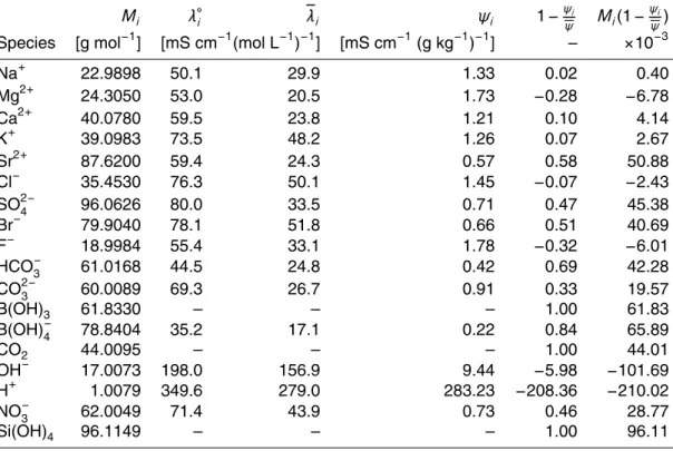
whereM_i (Table 2) is the molar mass of the ith of N_c components of seawater (not including dissolved gases), andci its concentration. This difference arises for historical

reasons (see, e.g., Millero et al., 2008, for more details). For SSW this difference can be accounted for by a simple scaling

SA=γS78 (3)

5

whereγ incorporates updated knowledge of the true chemical composition of SSW. However, for real ocean waters there are also small spatial and temporal differences in the relationship arising from small variations in the relative chemical composition of seawater. Thus in general:

S_A=γS78+δSA (4)

10

The offsetδSAis in the range of 0 to 0.03 g kg− 1

in the open ocean, with largest values in the North Pacific (McDougall et al., 2009), and can be as large as 0.05 g kg−1 in some estuarine waters (Millero, 1984).

In recent years the increasing number of high-quality conductivity measurements of seawater on global scales has led to the realization that these spatio-temporal

dif-15

ferences may have practical importance in understanding the global circulation. A reevaluation of the procedures for determining thermodynamic properties of seawater, including density, suggests that more accurate results can be obtained by returning to a procedure in whichS_A is used instead of S78 as a state variable (Feistel, 2008;

Millero et al., 2008). In this procedure a best estimateS_R for theS_Aof SSW is made by

20

takingγ=uP S≡35.16504/35≈1.004715. For non-standard seawaters an offsetδSA08,

found using an algorithm involving a geographic look-up table (McDougall et al., 2009), is added toS_R to calculateS_A08 as a best estimate forS_A.

SA can be directly estimated by measuring the density of water samples and then

inverting the equation of state which relates density and salinity. The algorithm for

25

S_A08 is based on a fit of such data against measured Si(OH)4 concentrations. Other

(5)

OSD

6, 2861–2909, 2009

model

R. Pawlowicz

Title Page

Tables Figures

◭ ◮

Back Close

Full Screen / Esc

These are also based on purely empirical correlations with concentrations of specific chemical species, typically nutrients and components of the carbonate system.

However, little work has been done on understanding the full theoretical basis for these corrections. A complete chemical theory would include a model for seawater, and a method for determining the variations in conductivity and density that result from

5

compositional variations. Density has been well-studied (e.g. Millero et al., 1976), but in spite of the practical importance of conductivity in ocean measurements there has been virtually no work done in developing a theory of electrical conductivity for nat-ural seawaters. Recently, a model has been developed for calculating the electrical conductivity of natural freshwaters, based on their chemical composition (Pawlowicz,

10

2008, hereafter Pa08). Although the Pa08 model works well for waters of low salinities (less than a few g kg−1of dissolved solids), accuracy in waters of higher salinities is not sufficient to directly replace the empirical relationship specified by PSS-78 (Pawlowicz, 2009). However, it will be shown here that the model can be used to quantitatively calculate the effects of small compositional variations on the known PSS-78

conductiv-15

ity/salinity relationship.

The purpose of this paper is then twofold. First, to develop a seawater conductiv-ity model, based on Pa08, capable of quantitatively determining the effects of small variations in the chemical composition of a model seawater on its conductivity, and consequently onS78. Second, to use this model to compute correctionsδSA directly 20

from a suitable set of observations, independent of density measurements. This model will then be a complement to the available empirical estimatesδS_A08.

2 Methods

The general approach is based on modelling perturbations about a known base state for SSW. The base state consists of the known PSS-78 relationship (Eq. 1), and a

25

chemical compositionCwhich is a function ofS78.

(6)

OSD

6, 2861–2909, 2009

model

R. Pawlowicz

Title Page

Tables Figures

◭ ◮

Back Close

Full Screen / Esc

practical salinity S78, true conductivity κ=f− 1

78 (S78), and computed absolute salinity S_A(C). The composition C will be based on a model of the changes arising from di-lutions and evaporations of a reference composition C0 for whichS78=35. Thus our

seawater model will mimic the seawater used to develop PSS-78, and can be used to estimateγ.

5

The second step is to compute conductivity and absolute salinity perturbations, δκ

andδArespectively, arising from compositional changes. There are two kinds of per-turbation possible. The most straightforward occurs when a known perper-turbationδcis added to the base stateC. The Pa08 conductivity model is used to estimate δκ. In this calculation a nonzero δS_A arises because both S_A and S78 change, but by dif-10

ferent amounts. Since these situations often involve composition changes only in the nonconservative elements of seawater, we call this a constant chlorinity calculation. However, estuarine situations when freshwaters (which may contain Cl− and other so-called conservative elements) are added will also be handled in this way. Results can be simplified into an approximate analytical form, which can then be used to

qualita-15

tively understand the effect of perturbations.

In contrast, a more formally correct procedure for the correction of ocean measure-ments is to compute δSA when the composition is perturbed, but κ (and hence S78)

are fixed. In this constant conductivity calculation the addition of a known concentra-tion of (say) nitrate, which is ionic and would increase conductivity, would be balanced

20

by a small dilution of the SSW composition. The Pa08 model is then used iteratively to calculate the dilution factor. A changeδSA=δAarises because the concentrations

of all components change. The two procedures provide nearly identical δS_A for the examples considered here.

Unless otherwise stated, all calculations are carried out for a temperature of 25◦C

25

(7)

OSD

6, 2861–2909, 2009

model

R. Pawlowicz

Title Page

Tables Figures

◭ ◮

Back Close

Full Screen / Esc

2.1 A composition model for standard seawater (S₇₈=35)

Typical oceanic concentrations of virtually all elements in the periodic table are now known (e.g., Nozaki, 1997), but many elements are present in only trace quantities. The model base state (labelled SSW76, see Columns 1-2 of Table 3) is meant to to match as closely as possible the composition of the North Atlantic surface seawater

5

circa 1976 used to derive both PSS-78 and the 1980 equation of state (Millero and Poisson, 1981). It includes all components that can affect salinity down to the level of 1 mg kg−1, although traditional practice in not including the dissolved gases N2

(16 mg kg−1), and O2 (0–8 mg kg− 1

) is followed. This composition is denoted by a vector C0={c1 c2 ... cNc}, where ci is the concentration (mol kg

−1

solution) of the

10

ith of Nc constituents. SSW76 is defined to have S78=35 (exactly), and constructed

to have a chlorinity of 19.374 g kg−1 according to the definition (Millero et al., 2008) derived from titration procedures:

Chlorinity/(g kg−1)≡0.3285234×MAg×([Cl−]+[Br−]+[I−]) (5)

with [·] denoting concentrations andMAg=107.8682 g mol− 1

the molar mass of silver.

15

In addition, the reference salinity SR≡uP SS78 (Millero et al., 2008), will be (exactly)

35.16504 g kg−1.

The recently defined reference composition of standard seawater (from Millero et al., 2008, hereafter M08) was taken as a starting point in specifying SSW76. However, M08 cannot easily be used directly as a model for seawater in this study for several

20

reasons.

First, the fixed ratios of carbonate system components in M08 are not convenient for studying spatial and temporal variations in seawater composition. Although speci-fication of the carbonate system in seawater requires (at minimum) 7 species (Millero, 1995), some of which appear in amounts much less than 1 mg kg−1, their

concen-25

(8)

OSD

6, 2861–2909, 2009

model

R. Pawlowicz

Title Page

Tables Figures

◭ ◮

Back Close

Full Screen / Esc

DIC}are required to fully specify the carbonate system (with minor corrections arising from borate and SO2₄− concentrations). From these parameters, the equilibrium con-stants (denoted by K_w,K0,K1,K2,KB and parameterized in Dickson et al. (2007)) are

used the compute the ionic concentrations.

It is desirable in the model to let the carbonate ions remain in chemical

equilib-5

rium in all conditions as this more closely models the behavior of real water. Thus instead of using the M08 ionic concentrations, the carbonate system is defined using two of the standard parameters. The first parameter used is Total Alkalinity (T A), set to 2300µmol kg−1, where

T A≡[HCO−₃]₊2[CO2₃−]₊[B(OH)−₄]₊[OH−]−[H+] (6)

10

A total borate component is specified by adding together the B(OH)−₄ and B(OH)3

com-ponents of M08, and SO2₄− concentrations (required for carbonate system calculations) are also taken from M08.

Second, although theT Aof SSW76 and M08 are the same, the total dissolved inor-ganic carbon (DIC) defined as

15

DIC≡[CO2]+[HCO−3]+[CO 2−

3 ] (7)

in the two models is different (as are pH andfCO₂). The reason for this is that attempts to matchδSAobservations, as well as weak independent evidence, suggests that the

DIC content of SSW is somewhat higher than that specified in M08.

M08 specifies ionic composition after setting the fugacity fCO₂ to 333 µ-atm at a

20

temperature of 25◦C. ThisfCO2is appropriate for an equilibrium with atmospheric

lev-els when the measurements were made to define PSS-78, and at 25◦C implies a DIC of 1963µmol kg−1. Typically, after sampling, SSW is filtered and sterilized for≈30 days at temperatures of 28◦C before 1991 (batch numbers up to P115), but only 18–21◦C since then (P. Ridout, OSIL, personal communication). Since the solubility of CO2 is 25

(9)

OSD

6, 2861–2909, 2009

model

R. Pawlowicz

Title Page

Tables Figures

◭ ◮

Back Close

Full Screen / Esc

be 1937 µmol kg−1. The change in DIC due to increasing atmospheric CO2 levels

is slightly smaller. At a temperature of 25◦C and a present-day fCO2 of 380 µ-atm,

calculated DIC would be 1992µmol kg−1.

However, there are indications that measured DIC values in ampoules of SSW are often (but not always) somewhat higher than these predicted equilibriums at bottling

5

time, and this is generally believed to be caused by the decomposition of residual organic matter after bottling. Unfortunately, although theT Aof standard seawater has been studied (Goyet et al., 1985; Millero et al., 1993), there has been no systematic attempt to analyze the DIC content of standard seawater, and its temporal stability. Brewer and Bradshaw (1975) measured 2238µmol kg−1 in SSW batch P61. Recent

10

(September 2009) measurements of DIC in ampoules of old SSW from batches P79 (from 1977), P111 (1989), and bottled P140 (2000) found values of 2610, 2200, and 1803µmol kg−1, respectively. The spread between replicates from different ampoules of the same batch was 10–20 µmol kg−1, larger than measurement uncertainty, but much smaller than the variations between batches.

15

In fact, as will be shown later, conductivity is not sensitive to variations in DIC, al-thoughS_A (and hence δS_A) are greatly affected. A DIC change of 100 µmol kg−1 is equivalent to an absolute salinity variation of ≈0.006 g kg−1, but will change S78 by

only 0.0007. Since a primary purpose of ourδSA corrections is (eventually) to

calcu-late densities, it may be more important to choose a model DIC value that will match

20

that of the water used in the measurements defining the 1980 equation of state (Millero and Poisson, 1981), relating salinity and density. This is stated by Millero (2000) to have been 2226µmol kg−1. However, density fits to Pacific ocean data published in that paper also suggest zero density anomalies occur when DIC=2000µmol kg−1.

Since ampoules of SSW are sealed, this large range of uncertainty is ultimately

re-25

(10)

OSD

6, 2861–2909, 2009

model

R. Pawlowicz

Title Page

Tables Figures

◭ ◮

Back Close

Full Screen / Esc

desirable that our definition (eventually) imply that δS_A≈0 for observations from the surface North Atlantic. Thus, after some tuning, DIC is set to 2080µmol kg−1.

An inappropriate value for the DIC of SSW76 will (eventually) lead to a near-constant offset in all calculated absolute salinity variations. Although this offset is thus potentially significant, it will apply to all calculations and hence may have little effect on

compar-5

isons between different seawaters, or on any computation in which additions rather than absolute levels of DIC are specified.

The last difference is that non-conservative nutrient species must be included. Changes in NO−₃ and Si(OH)4will exceed 1 mg kg

−1

in a seawater withSA≈35 g kg−1

and are related to the salinity variations we seek to model (Brewer and Bradshaw,

10

1975; Millero, 2000). These nutrients are assumed to have a concentration of zero in SSW76.

Following customary practice the mass of Na+is adjusted slightly to maintain charge neutrality, once all other ionic components are specified in SSW76. This may partly ac-count for the contributions of neglected ionic constituents, of which the most important

15

are the conservative elements Li+ (0.18 mg kg−1, Soffyn-Egli and Mackenzie, 1984), Rb+ (0.12 mg kg−1), and the nutrient PO−₄ (0–0.23 mg kg−1).

The computed absolute salinity S_A(C₀)=35.171 g kg−1 for SSW76. This differs by 0.006 g kg−1 from the defined value ofSR. The mismatch is within the uncertainty of

±0.007 g kg−1 suggested by Millero et al. (2008), however much of that error arises

20

from uncertainty about the amount of SO2₄−. In contrast, the salinity difference here largely arises from di_fferences in carbonate parameters. However, it should be em-phasized that SSW76 is a model of seawater, and not necessarily a better (or worse) description of actual seawater than M08. This is because the assumed precision for some of the constituent concentrations that is greater than that of the best

observa-25

tions.

Strictly speaking, the difference betweenγ=35.171/35 andu_{P S} means that theδS_A

computed in this paper, needed to get true absolute salinity SA, is not exactly the

(11)

OSD

6, 2861–2909, 2009

model

R. Pawlowicz

Title Page

Tables Figures

◭ ◮

Back Close

Full Screen / Esc

corrections will be related by a scale factor ofγ/uP S≈1.00017. However, the difference

is small enough that it is not of any practical importance and the two will be considered interchangeable.

2.2 A model for standard seawater (S786=35)

The composition of waterCat salinities other thanS78=35 can be specified in different 5

ways. The simplest is to multiply all constituent concentrations by a constant fraction (i.e.C(3)=β×C0forS78=β×35). This is a so-called type III Reference Seawater (Millero

et al., 2008). However, during the specification of PSS-78, SSW was evaporated or di-luted with distilled water in order to change its salinity, and again equilibrated with the atmosphere. This makes it more reasonable to specify a type II Reference Seawater

10

C(2), where only the concentrations of conservative tracers, as well as T A, are multi-plied by the constant fractionβforS78=β×35, butfCO2is kept constant.

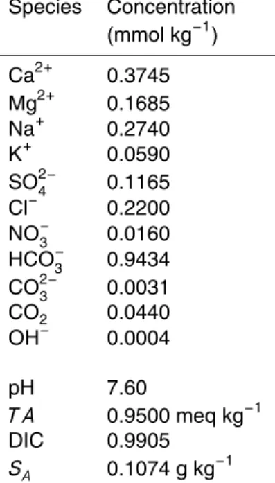
Assuming in advance of our later discussion that the conductivity model can pre-dict the effects of perturbations reasonably well, and realizing that C(2) and C(3) are very similar, the differences in conductivity, absolute salinity, and conductivity-derived

15

practical salinity arising from these two approximations can be estimated as:

δκ′=κ_{P a08}(C(2)₎₋_κ

P a08(C(3)) (8)

δS_A′ =S_A(C(2))−S_A(C(3)) (9)

δS₇₈′ =f78(κP a08(C(2)))−f78(κP a08(C(3))) (10)

whereκP a08 is the conductivity estimate computed using the Pa08 conductivity model 20

and absolute salinities are calculated using Eq. (2).

Over the range of 5<S78<40, the conductivity differences are δκ′<±0.8 µS cm− 1

(Fig. 1a), which in turn impliesδS₇₈′ <±0.0005 (Fig. 1b). These uncertainties are negli-gible. However, the changes in absolute salinityδS_A′ are an order of magnitude larger, and can approach 0.004 g kg−1 at salinities of about 17 (Fig. 1b) although the diff

er-25

(12)

OSD

6, 2861–2909, 2009

model

R. Pawlowicz

Title Page

Tables Figures

◭ ◮

Back Close

Full Screen / Esc

2.3 A perturbation model for observed seawater

As a particular parcel of seawater is advected through the ocean within the thermoha-line circulation, biogeochemical processes alter its composition so it differs from that of SSW. These perturbations are represented by a vectorδc, so that the composition be-comesC+δc. Biogeochemical processes will not alter the conservative components

5

of seawater, so these components of δc are zero. Changes occur due to variations in non-conservative nutrients and components of the carbonate system. However, cal-culations appropriate for estuarine waters may also involve changes in some of the conservative components as they may also be components of freshwaters.

Note that a slight simplification has been made. Actual additions of a particular

10

species to a volume of water will (slightly) change the concentrations of all other species, when concentrations are measured per unit mass of solution (or per unit vol-ume) as is done here. However, modelling this additional complication is not necessary here as we are not tracking individual parcels.

Nutrient changes that lie above our threshold of 1 mg kg−1include nitrate (NO−₃) and

15

silicate. The latter can appear in the form of SiO₂, Si(OH)₄, and SiO(OH)−₃. Typically in the pH range of seawater all but a few percent appears as nonconductive Si(OH)4, and

it will therefore be assumed that only a negligible amount appears in the other forms. Changes to the carbonate system can be determined by measurements of T Aand DIC (or any two equivalent measurements, e.g. pH andT A). With the addition of NO−₃,

20

and a change inT A, the number of positive and negative charges in the composition will probably no longer balance. Other processes must therefore be present in the real ocean to balance this excess (or rather, the change in T A arises to compensate for the effects of these other processes). The dissolution of CaCO3 is likely the

predom-inant mechanism at work (Sarmiento and Gruber, 2006). The negative charges and

25

(13)

OSD

6, 2861–2909, 2009

model

R. Pawlowicz

Title Page

Tables Figures

◭ ◮

Back Close

Full Screen / Esc

a relationship between the increase in TA and the increase in concentrations of Ca2+ from dissolution and NO−₃ from remineralization:

∆T A=2∆[Ca2+]−∆[NO−₃] (11)

where∆ denotes changes. Thus our perturbations must include measured concen-trations of NO−₃, Si(OH)₄,T A, and DIC, as well as an inferred change in Ca2+ using

5

Eq. (11). Carbonate parameters are then recomputed using the equilibrium constant formulas described by Dickson et al. (2007).

Of course, other processes also occur in the ocean. For example, T A also varies with changes in phosphate and organic substances, although these contributions will fall below our threshold of importance. A more important process might be sulfate

10

reduction on continental shelves (Chen, 2002), which may be responsible for a large part ofT Aincreases in some areas. In order to model this situation Eq. (11) would be modified to:

∆T A=2_∆[Ca2+]−2_∆[SO2₄−]−∆[NO−₃] (12) but now an additional relationship (specifying, e.g., the importance of CaCO3 dissolu-15

tion relative to SO2₄− reduction) is needed to complete the model. Speculation on this relationship is beyond the scope of this paper.

There is also evidence for significant (relative to our threshold) variations in the con-centrations of Mg2+in the vicinity of hydrothermal vents (de Villiers and Nelson, 1999). Again, the wider importance of this process, and a means of parameterizing these

20

variations, is at present unknown.

2.4 A model for seawater conductivity

The Pa08 model estimate κPa08 of the true electrical conductivity κ of a dilute

(14)

OSD

6, 2861–2909, 2009

model

R. Pawlowicz

Title Page

Tables Figures

◭ ◮

Back Close

Full Screen / Esc

can be written in a simplified form as (Pawlowicz, 2008)

κPa08(C)= N_c

X

i=1

λ_ic∗_iz_i (13)

The in-situ ionic equivalent conductivitiesλ_i=λ◦_if_iα_i are the product of infinite dilution equivalent conductivitiesλ◦_i for the different ions (set to zero for nonionic species), and two reduction factors: fi(I∗)≤1, accounting for relaxation and electrophoresis effects, 5

and α_i(I∗,C)≤1, accounting for ion association effects at finite ionic strength I∗. The stoichiometric ionic strengthI∗is

I∗=1 2

Nc

X

i=1

z_i2c∗_i (14)

The valence of charge on the ith ion is zi and its stoichiometric concentration c∗i

(mol L−1). This is related toc_i through a density equation (Millero and Poisson, 1981):

10

c∗_i =ρ(S78)ci (15)

where we incur an error of at most 1×10−5by ignoring the fact that the true density will change slightly with composition perturbationsδc. AsI∗→0 we havefi→1 andαi→1.

The relaxation/electrophoresis reduction parameter fi for speciesi depends on the

concentrations of other speciesj6=i only through their contribution toI∗. However, the

15

ion association parameterα_i depends critically on the concentrations and identities of all other ions (i.e. on the total set ofc∗_i,i=1,...,Nc), as it is a weighted sum of

interac-tions with all other anions (cainterac-tions) for a cation (anion). In order to account for this the internal model structure is somewhat more complicated than Eq. (13) suggests. Both the infinite dilution equivalent conductivities, and the in-situ ionic equivalent

conductiv-20

ities determined by Pa08 for SSW76, are listed in Table 2.

(15)

OSD

6, 2861–2909, 2009

model

R. Pawlowicz

Title Page

Tables Figures

◭ ◮

Back Close

Full Screen / Esc

parameters are based purely on basic chemical measurements in binary solutions, without reference to any measurements made in seawater (or any other natural water). The accuracy of the computed conductivity κPa08 depends on the accuracy of the

measured ionic concentrationsc∗_i, as well as on biases in the calculation of the reduc-tion factors fi and αi. At salinities<4g kg−

1

the relative accuracy ε=(κP a08−κ)/κ of 5

the model is typically limited to±0.03 by the accuracy of the chemical analyses used to determine composition (Pawlowicz, 2009). Once this error is reduced, by, e.g., statisti-cal averaging, the true error is less than 0.007 over a range of chemistatisti-cal compositions. For seawater with salinities of 0.1–1 g kg−1 we find an overestimate of only 0.002. However, at the higher salinities of concern here model biases dominate the error, with

10

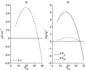
εsmoothly varying from about−0.01 at a salinity of 4 (κ∼8 mS cm−1) to about−0.10 at a salinity of 35 orκ∼50 mS cm−1(Fig. 2b).

2.5 Conductivity perturbations for non-standard seawaters

A salinity underestimate of order 3 g kg−1resulting from using κPa08 in Eq. (1) directly

will not allow us to directly investigate the small compositional variations in typical

sea-15

water that we have discussed above, which are several orders of magnitude smaller. However, not only is|ε|≪1, but it is relatively insensitive to changes in chemical com-position. A comparison of measured and predicted conductivities for a variety of saline ocean and lake waters in the range of 20-50 mS cm−1 (Fig. 2b) shows that the result-ing error is virtually identical for different compositions at the same conductivity. This

20

is very different from results found when considering baseline predictions formed by takingfi=αi=1, or equivalently using infinite dilution equivalent conductivities for the

different components, ignoring all interionic interactions (Fig. 2a). Not only are these baseline predictions greatly in excess of true conductivities (so thatε=O(1)), but the ex-cess is highly sensitive to the composition. The baselineεfor Mahoney Lake is almost

25

(16)

OSD

6, 2861–2909, 2009

model

R. Pawlowicz

Title Page

Tables Figures

◭ ◮

Back Close

Full Screen / Esc

Thus for model predictions during which only small changesδc in composition are made, we can take theκPa08 errorε≈constant. εis estimated from

κ(C)=κPa08(C)·(1+ε)−1 (16)

knowing thatκ(C)=f₇₈−1(S78). Since we assume

κ(C+δc)≈κPa08(C+δc)·(1+ε)−1 (17)

5

the change in conductivityδκ related to small compositional changes is:

δκ≡κ(C+δc)−κ(C)

≈(κPa08(C+δc)−κP a08(C))·(1+ε)−1

=δκPa08·(1+ε)−1 (18)

Thus it appears that we can use Pa08 to usefully predict conductivity perturbations.

10

We can confirm the relationship postulated in Eq. (18) for Pa08, which suggests that increments will be modelled to the same relative accuracyε as conductivities them-selves, by directly comparing numerical estimates from the model of various deriva-tives and other parameters related to conductivity increments with observations made in seawater.

15

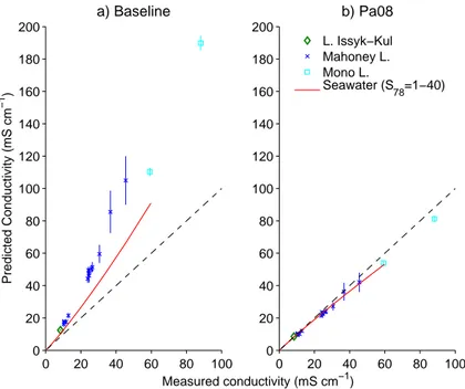
First, direct estimates of the ionic equivalent conductivitiesλi=λ◦ifi in seawater have

been made using a radioactive tracer technique (Poisson et al., 1979). These parame-ters can also be extracted from the Pa08 model. When using the baseline (i.e. ignoring all modelled ionic interactions) the parameters are overpredicted with relative errors of 0.34 to 1.5 (Fig. 3a). However, when using the full Pa08 model, predictions are

20

much closer to measured values, and the scatter is also greatly diminished. The mean relative error is−0.09, almost identical to that found for conductivity itself.

Note that although the equivalent conductivities are generally underpredicted, the results for SO2₄− show a slight overprediction. This ion associates strongly with most other cations. This makes it more difficult to model the equivalent conductivity of the

25

(17)

OSD

6, 2861–2909, 2009

model

R. Pawlowicz

Title Page

Tables Figures

◭ ◮

Back Close

Full Screen / Esc

the error when making predictions in actual solutions, as pairing effects are added back in.

More relevant results can be obtained by comparison with so-called partial equivalent conductivitiesΛ1i, defined by

Λ1i= ∂κ ∂E_i

_P,T,E

j6=i,...

(19)

5

These have been evaluated from laboratory measurements in which small changes in equivalent concentrationsE_i of theith of the N_s salts (i.e. binary compounds) in sea-water are made by additions to a reference seasea-water (Park, 1964; Conners and Park, 1967; Conners and Weyl, 1968; Conners and Kester, 1974; Poisson et al., 1979). The data are corrected to show the derivatives when all other other conditions, and

concen-10

trations of all other ions, are held fixed. Note that theΛ1i are not equal to the sum of

the corresponding equivalent conductivities for the anion and cation in Eq. (13) when evaluated at the ionic strength of seawater. Differences arise due to changes in the ionic strength, and in the effects of pairing (i.e., when α<1) between the components of the added salt and all other constituents in seawater. However, theΛ1i can easily 15

be computed numerically from the Pa08 model.

For the salts studied, baseline predictions overestimate the partial equivalent con-ductivities by 0.46 to 3.4 (Fig. 3b and c). When using the full Pa08 model, predictions are much closer to measured values, and the scatter is also greatly diminished (mean relative error−0.12). We also see that added salts containing SO2₄−tend to lie close to

20

(18)

OSD

6, 2861–2909, 2009

model

R. Pawlowicz

Title Page

Tables Figures

◭ ◮

Back Close

Full Screen / Esc

2.6 Salinities of non-standard seawaters

The change inS78 resulting from a perturbationδcis given by

δS78 ≡S78(C+δc)−S78(C) (20)

=f78(κ(C+δc))−f78(κ(C)) (21)

≈f78(κ(C)+δκPa08·(1+ε)−1)−f78(κ(C)) (22)

5

whereεandδκPa08are as defined in the previous section. At low salinities whereκPa08

has minimal bias the simpler approximation

δS78≈δS78∗ ≡f78(κPa08(C+δc))−f78(κP a08(C)) (23)

provides an alternative method of estimatingδS_Awhich does not rely on assumptions about the magnitude of perturbations. In fact the functionf₇₈(κ) is smooth enough that

10

the approximation holds to a degree of accuracy ≪ε over all salinities (c.f. Eq. 10), although we continue to use the computationally more intensive Eq. (22) unless oth-erwise specified. In addition to these changes in S₇₈, perturbations δc also lead to changes inSA according to:

δA≡S_A(C+δc)−S_A(C)=S_A(δc) (24)

15

(by the linearity of Eq. 2).

If we consider a parcel of water with fixed chlorinity, additionsδcwill therefore affect both the measuredS₇₈ and calculatedS_A. These changes will generally be different, giving rise to a salinity correction which can be estimated as:

δS_A∗ ≡S_A(C+δc)−γS78(C+δc) (25)

20

=δA−γδS78 (26)

≈δA−δS78 (27)

(19)

OSD

6, 2861–2909, 2009

model

R. Pawlowicz

Title Page

Tables Figures

◭ ◮

Back Close

Full Screen / Esc

dominate the correction. On the other hand, adding very light but extremely conductive ions could lead to negative corrections arising mostly from changes inS78.

However, when converting ocean measurements to absolute salinity we are con-cerned with the corrections that arise whenS78 is held constant, rather than those for

fixed chlorinity. For non-standard seawater with a measuredS78 the composition is not 5

Cbut ratherβC+δc. That is, the addition of other solids that dissociate into ions which increase conductivity must be matched by a slight dilution of our standard seawater composition in order to keep conductivity constant. The dilution factorβfor the SSW composition can be found by solving

κ(βC+δc)=κ(C) (28)

10

which can be done iteratively, usingκPa08 in place ofκ on both sides of the equation.

Then from Eqs. (4) and (28) the true correction is:

δS_A=S_A(βC+δc)−S_A(C)=δA−(1−β)S_A(C) (29)

Typicallyβis very close to 1 andδS_A∗ is within a few percent ofδS_Afor the small pertur-bations of concern here. Although the latter is technically more correct, the advantage

15

of the former is that we can separately estimate effects of changing mass and changing number of electrical charges.

3 Results

To illustrate the effects of compositional changesδcfirst consider an extreme, but re-alistic, scenario. Investigations of the relationship between salinity and density suggest

20

that largest δS_A (of order 0.03 g kg−1) occur in the intermediate North Pacific (Mc-Dougall et al., 2009). This water represents the endpoint of the subsurface branch of the thermohaline circulation and thus provides an appropriate extreme. For com-parative purposes model “North Pacific Intermediate Water” (NPIW) is normalized to have the same chlorinity as SSW76, although actual chlorinities in the North Pacific

(20)

OSD

6, 2861–2909, 2009

model

R. Pawlowicz

Title Page

Tables Figures

◭ ◮

Back Close

Full Screen / Esc

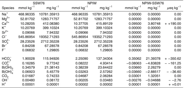
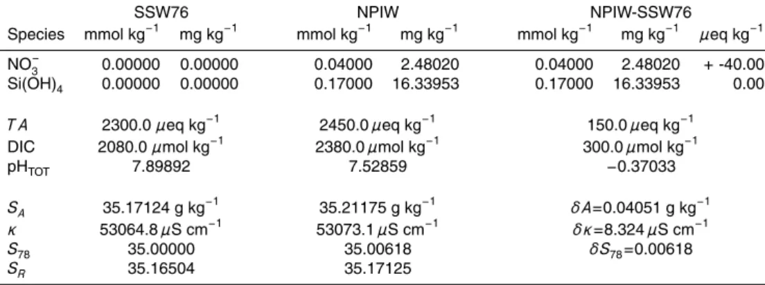
are about 0.3 g kg−1 lower. Based on typical observations, take this water to con-tain Si(OH)4=170 µmol kg−

1

and NO−₃=40 µmol kg−1, with T A and DIC larger than in SSW76 by values of 150 µeq kg−1 and 300 µmol kg−1 respectively. Columns 4– 5 of Table 3 then contain the model compositionC0+δc representing NPIW, with the

perturbationδcin columns 6–8.

5

Carbonate equilibria are recalculated from the new T A and DIC. pH on the Total scale drops to about 7.5 (again, all calculations are at 25◦C). The increases we specify actually cause concentrations of CO2₃− and B(OH)−₄ to decrease significantly. In addi-tion, charge balance considerations require that the concentration of Ca2+ increase by 0.095 mmol kg−1or a little less than 1% over its value in SSW76. Measured increases

10

inCa2+ at depth in the North Pacific are of this order (de Villiers, 1998).

Applying the model directly (i.e. under conditions of fixed chlorinity) δS₇₈≈0.0062 and δA≈0.0405 g kg−1, and hence from Eq. (27) δS_A∗≈0.034 g kg−1. The cruder approximation δS₇₈∗ ≈0.0054 underestimates δS_A with a relative error of only -0.12. A similar calculation, i.e., one with the same changes inT A, DIC, NO−₃, and Si(OH)₄,

15

under conditions of fixed conductivity, results in a dilution factor ofβ=0.9998105, and from Eq. (29)δS_A≈0.034 g kg−1.

The two calculations result in almost exactly the same answer. From Eq. (27) we can consider the correction as the difference between changes in absolute and prac-tical salinity. The Si(OH)4 component alone contributes about 0.016 g kg−

1

toδS_A, or

20

almost half of the correction. Much of the remainder arises primarily due to increases in HCO−₃, but there are both increases and decreases in other constituents. In fact, the changes inS_A due to the increase in carbonates outweigh those due to the increase in Si(OH)₄, but some of this carbonate ion increase is compensated by an increase in

S78. 25

(21)

OSD

6, 2861–2909, 2009

model

R. Pawlowicz

Title Page

Tables Figures

◭ ◮

Back Close

Full Screen / Esc

with the exception of H+ and OH− are all of order 30 mS cm−1 (mol L−1)−1. Very roughly then, conductivity changes will be proportional to changes in the number of charge pairs present. There are large changes in the concentrations of individual neg-ative ions (last column of Table 3), but overall the increases and decreases in negneg-ative ions tend to balance out, matching (in total) the smaller increase in positive charges

5

from Ca2+ produced by CaCO₃ dissolution. Thus changes in SA are most strongly

influenced by changes in Si(OH)4 and DIC, but changes in S78 occur mostly due to

CaCO3dissolution.

Further insight can be obtained by deriving an approximate relationship between

δS_A and δc. Seawater conductivity per unit mass of salt at 25◦C in the model is

10

ψ=κPa08/SA≈1.35 mS cm− 1

(g kg−1)−1. Combining Eqs. (2), (4), and (13) and defining

ψi=λiziρ/Mi as the conductivity per unit mass of theith component:

δS_A≈X

i

M_i(1−ψi

ψ)δci (30)

with numerical values appropriate forS78=35 given in Table 2. This expression

illus-trates the way in which the contribution of individual ions toδS_Adepends on the degree

15

by which conductivity per unit massψ_i differs from the averageψ. The relationship is only approximate because theψ are not in fact constant, but will also vary withδc. In using this formula it is also important to recall that only charge balanced perturbations are meaningful, so that any scenario must involve changes in at least one cation and anion.

20

Examination of the mass effect coefficients (1−ψi/ψ) for different ions (listed in

Col-umn 6 of Table 2) shows concentration perturbations in some ions (e.g., Na+, Ca2+, Mg2+, K+, Cl−, F−) result in little change to δS_A. These ions contribute to conduc-tivity in an “average” way, withψi≈ψ. Contrariwise, concentration changes in other

ions do not affect conductivity in an average way and hence must be accounted for

25

(22)

OSD

6, 2861–2909, 2009

model

R. Pawlowicz

Title Page

Tables Figures

◭ ◮

Back Close

Full Screen / Esc

processes. Nonconductive species contribute exactly their added mass. Several ions (H+, OH−) have an extremely large effect on conductivity, relative to their mass. How-ever, the actual in-situ mass changes in these ions are so small that the overall effect on conductivity is minimal.

Seawater is composed primarily of Na+ and Cl− ions (Table 3). These contribute to

5

conductivity in an average way, and so if there are small perturbations in their mass

S₇₈ will approximately account for the salinity change. When using the full model, and ignoring nonconductive Si(OH)4, the change in absolute salinity δA is ≈0.024,

about 4 times larger thanδS78. However, our salinity perturbation for modelling NPIW

is composed largely of HCO−₃, for which ψ_i is significantly different than ψ. Using

10

Eq. (30) we expect that an HCO−₃ perturbation will give rise to a conductivity change that (when converted to salinity using the average factorψ) will only account for≈0.3 of the actual salinity change. The dominance of HCO−₃ changes inδc, and their relatively unconductive nature, explains the insensitivity of predicted conductivity to variations in our assumptions about how seawater dilution should be modelled (c.f. Sect. 2.2).

15

The choice between Eqs. (11) and (12) to balanceT Achanges will also have some consequences. An addition of Ca2+ will result in a compensating increase in conduc-tivity, not affectingδS_A, but an equal decrease of SO2₄− (which has an equivalent effect onT A) will not result in a fully compensating decrease in conductivity and hence will result in a smaller δSA. For a concentration change of order 100 µmol kg−1 (i.e. for 20

NPIW) the difference in δS_A computed using the different scenarios is 0.005 g kg−1 using Eq. (30) or 0.008 g kg−1 using the full model. Since we do not have a good knowledge of the actualδci for all constituents of seawater, we must rely on

assump-tions about biogeochemical processes to parameterize them. However, our prediction accuracy is then limited by the extent of our knowledge about these processes.

25

By considering only those ions both important in typical biogeochemical perturba-tions (i.e. large values in column 7 of Table 3) and with strong effect onδSA (i.e., with

(23)

OSD

6, 2861–2909, 2009

model

R. Pawlowicz

Title Page

Tables Figures

◭ ◮

Back Close

Full Screen / Esc

onδSA. Since all of the carbonate parameters are related, and relationships such as

Eq. (11) mean that the NO−₃ term is not really independent either, a more sophisticated understanding of the carbonate system may allow a formula forδS_Ato be written more simply in terms of more general parameters such asT Aand DIC.

However, for accurate calculations the full model is required. Unfortunately, although

5

our model can be used to directly compute δS_A in any situation, the computational process by which these values are derived is complex and relatively opaque. Previous workers have fitted simple empirical relationships to measurements, and these appear to be sufficient for practical purposes. Such formulas can also be fitted to “measure-ments” calculated by the perturbation model. This is a simpler way to derive more

10

straightforward formulas.

First consider perturbations whenS78=35. The model is used to calculateδSAover

a grid ofδc points within a range of 0≤∆T A≤0.3 meq kg−1, 0≤∆DIC≤0.3 mmol kg−1, and 0≤∆NO−₃≤0.040 mmol kg−1, with Ca2+ again varying according to Eq. (11). In-spection of the results shows thatδS_Avaries quasi-linearly with the components of the

15

perturbation, and by least-squares fitting the equation

δSA/(g kg−1)=(47.11∆DIC+7.17∆T A+36.57∆[NO−3])×10

−3 ₍₃₁₎

agrees very well with the full calculations, with a misfit standard error of

±0.00007 g kg−1and a maximum misfit of 0.0003 g kg−1.

The DIC coe_fficient is similar to the theoretical coe_fficient for HCO−₃ (Column 7

Ta-20

ble 2), and both the theoretical and fitted NO−₃ coefficients are roughly comparable. The ≈20% difference results from both the biogeochemical relationships, as well as variations in the interionic interactions involved in conductivity.

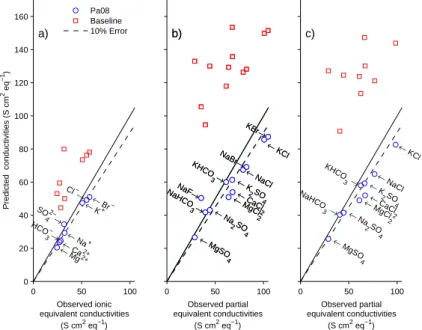
Repeating the above procedure for 25≤S78≤40, we find that the coefficients in the

fit for δS_A vary with salinity (Fig. 4). The coefficients for ∆DIC and NO−₃ vary only

25

(24)

OSD

6, 2861–2909, 2009

model

R. Pawlowicz

Title Page

Tables Figures

◭ ◮

Back Close

Full Screen / Esc

that Eq. (31) should be modified for situations when S786=35 by replacing ∆T A with

∆T A×S78/35. Note that the∆signifies the change from SSW values at the specified

salinity, e.g. the difference between observed T A and 2300×S78/35 µmol kg− 1

. We also add in the total mass of Si(OH)₄to produce this final prediction formula:

δS_A/(g kg−1)=(47.11∆DIC+7.17(S78/35)∆T A+36.57∆[NO−₃] (32) 5

+96.11∆[Si(OH)4])×10−3

Note that there may be no easy way to empirically verify the di_fferent coe_fficients with ocean measurements. An empirical fit to data has resulted in the following relationship

δSA/(g kg−1)=(50.13(∆NT A−0.215)+63.10∆[NO−3]+96.30∆[Si(OH)4])×10−3 (33)

(Millero, 2000, eq. 3) which has a similar coefficient for Si(OH)4, but otherwise is nu-10

merically somewhat different. However, the different constituents included are strongly correlated in the ocean. A least-squares fit to a restricted set of actual observations may therefore be rather insensitive in certain directions of the parameter space of co-efficients. Thus it is most appropriate at this stage to compare these different formulas only by examining their effect on measured ocean profiles.

15

The full calculation procedure can easily be applied to actual ocean profiles, as long as they include observations of S78, T A, DIC, Si(OH)4 and NO

−

3. These parameters

are now considered to be standard for deep-ocean hydrographic observations so no modification is needed in routine procedures. The latter 4 are enough to specify the non-conservative elements, with changes in Ca2+ inferred from Eq. (11) to maintain

20

charge neutrality.

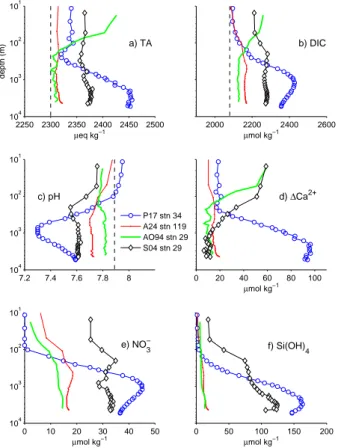
As an example, consider several recent high-quality hydrographic profiles from the North Atlantic, Arctic, and North Pacific, and Southern Ocean (Fig. 5–7). PreviousδS_A

estimates have been made in all regions except the Arctic.

Surface nutrients are low in all profiles except in the Southern Ocean, and surface

25

(25)

OSD

6, 2861–2909, 2009

model

R. Pawlowicz

Title Page

Tables Figures

◭ ◮

Back Close

Full Screen / Esc

Interactive Discussion T A, and DIC at depth are much higher in the North Pacific than in the other profiles.

However, deep pH is much lower. Deep nutrient levels are typically higher than surface nutrients in all cases. Inferred∆Ca2+ is high in the Arctic and Southern Ocean, and high in the deep North Pacific.

The computed salinity correctionδSAis close to zero in the surface waters of the N. 5

Pacific (Fig. 6a) and N. Atlantic (Fig. 6b), but is almost 0.008 in the surface waters of the Arctic (Fig. 6c). On the other hand, the correction is lowest at depth in the Arctic (only 0.003), but is as high as 0.033 in the deep North Pacific. The surface correction is highest in the Southern Ocean. The correction itself is dominated by theδ_A in all cases withδS_A≈0.8δA. The increase in ionic content does result in a small change in

10

conductivity which partially compensates for the compositional change, but as before

δS78≪δA.

Comparison of calculatedδS_Awith those produced by Eq. (33) and McDougall et al. (2009) for these stations are relatively good (Fig. 7). The general shape of depth profiles and overall magnitudes are similar, although our estimates appear to be

sys-15

tematically slightly larger. Correction factors in the deep Pacific and shallow Arctic are large, whereas theδSAare small in both Pacific and Atlantic surface waters, and deep

Arctic waters. Our corrections are about 0.005 larger in the deep Pacific and not very different whenδS_A≈0. Widest disagreement between the three estimates occurs in the Southern Ocean. For all profiles, the modelδSA is the largest of the 3 estimates, and 20

the predictions of McDougall et al. (2009) the smallest.

As a final comparison, the model is used to replicate the measurements in a con-trolled situation where the chemistry is more precisely known. Millero (1984) measured

δS_A (Fig. 8) for various mixtures composed of a known fractiona of SSW and an arti-ficial river water of known compositionC_R (Table 4):

25

Cmi xture=aC0+(1−a)CR (34)

(26)

OSD

6, 2861–2909, 2009

model

R. Pawlowicz

Title Page

Tables Figures

◭ ◮

Back Close

Full Screen / Esc

a perturbation in a fixed-chlorinity calculation. The name is somewhat misleading here because the river water also contains Cl− but this does not a_ffect the mathematical details of the calculation. Calculations must be modified slightly whenS78<5, since the

usual seawater parameterizations of the carbonate equilibria are no longer valid in this low-salinity range. They do not extrapolate correctly to pure-water limits. Instead we

5

use low-salinity parameterizations more suitable for river and lake waters (Pawlowicz, 2009; Millero, 1995). The change ofδS_Aacross the transition between the two regimes is not smooth, but the size of the step is small enough that it cannot be seen in Fig. 8.

TheδS_A∗ arising from perturbation computations almost exactly lies within the scatter of the observations (Fig. 8). As salinity drops and the riverine addition becomes a

10

larger fraction of the composition,δS_A∗ increases. One unexpected result is that δS_A∗

increases roughly linearly with decreases in salinity only at high salinities. WhenS_R

drops below about 10 g kg−1,δS78curves upwards quite sharply, so that theδSA∗ curve

flattens and even decreases at very low salinities. The observations do not appear to show this, although their scatter is large enough that this behavior cannot be ruled out.

15

However, at low salinities where the Pa08 model is known to be accurate (Pawlowicz, 2009), it can be applied directly to C_mixture and the alternative estimate δS₇₈∗ used in place of the perturbation calculation for δS78. Results agree almost exactly with the

perturbation model, showing the same curvature. Agreement is good at low salinities because the bias in Pa08 is small, and is good at high salinities because the river water

20

perturbation is very small.

Finally, fora=0 Pa08 directly predicts a conductivity of 142µS cm−1, which can then be used with PSS-78 to computeS78=0.0686 and hence δSA=0.0388 g kg−

1

inde-pendently of the seawater perturbation model. The perturbation model does approach these values in the limit asa→0. Note however that this limit is not a good indicator

25

of the zero-salinity intercept of a best-fit line through the observations, especially those from salinities>5 g kg−1, typical of most estuarine waters, because of the curvature in

δS78. Such a best fit line would intercept the left axis at rather higher values. Overall,

(27)

OSD

6, 2861–2909, 2009

model

R. Pawlowicz

Title Page

Tables Figures

◭ ◮

Back Close

Full Screen / Esc

different errors than those associated with riverine dilutions, there do not appear to be any general biases present.

4 Discussion and conclusions

The combination of a chemical model of seawater and a conductivity model allows the effects of compositional perturbations on conductivity-based methods of salinity

deter-5

mination to be estimated. An immediate result is that conductivity itself is relatively insensitive to biogeochemical perturbations to the chemical composition of seawater. In fixed chlorinity calculations, δS78 increases by less than 0.007 over the range of

waters investigated in the world ocean, whileS_A increases by up to 0.04 g kg−1. Nu-merical values of SR (i.e. the scaled S78) lie somewhere between a chlorinity-based 10

measure and the true absolute salinity, although much closer to the former. This also accounts for the stability of conductivity in SSW (Bacon et al., 2007), in spite of the known variations in DIC that occur within samples.

A second result is that the observedδSA are almost entirely explained by changes

in nutrients and the carbonate system. Although this fact is already known empirically

15

and is the basis for existing estimates of δS_A (e.g., McDougall et al., 2009; Millero, 2000) the model calculations provide a more theoretical confirmation. In addition, the model shows that variations in Ca2+and/or SO−₄ are as important as changes in NO−₃, although they are linked via biogeochemical relationships.

Another result is that the e_ffects of perturbations at typical oceanic salinities are

20

approximately linear functions of salinity, but that this linear behavior does not extrap-olate well to behavior at low salinities (S78<5). At low salinities carbonate composition

and δS78 become much more nonlinear functions of salinity. Thus generalizations

based on infinite dilution quantities, or river endpoints, are qualitatively useful but may in practice be less relevant to oceanic situations than might be otherwise be expected.

25

(28)

OSD

6, 2861–2909, 2009

model

R. Pawlowicz

Title Page

Tables Figures

◭ ◮

Back Close

Full Screen / Esc

However, although the general agreement between calculated δS_A and density-based estimates likeδSA08 is good, differences remain. The differences are not very

much larger than the typical uncertainty arising from density measurements, but are systematic. There are several possible explanations for these differences.

First, the Pa08 conductivity model may be inadequate to correctly calculate

pertur-5

bations in this application. The scatter in comparisons between predictions and ob-servations in Fig. 3 suggests that the model bias may still depend to some extent on chemical composition. It is difficult to fully address this issue without more data for com-parison. However, the good agreement with the dataset on mixtures of artificial river water and seawater (Fig. 8) suggests that model performance is adequate in at least

10

some cases, even when the perturbations become very large. Agreement between the fixed chlorinity calculation forδS_A∗ (Eq. 27) and the fixed conductivity calculation for

δS_A(Eq. 29) for the case of biogeochemical perturbations is also very good. The maxi-mum difference between the two is only 0.0007 g kg−1. Since each calculation involves somewhat di_fferent changes to the chemical composition, and di_fferent assumptions

15

about bias correction, this also suggests that these composition-dependent model er-rors are almost an order of magnitude smaller compared to the differences between model-estimated and density estimatedδSA.

Second, the overall comparison between the model and the other predictions in Fig. 7 can (perhaps) be improved by decreasing all calculatedδS_Aby a small (constant)

20

amount. Differences between the predictions will then be both positive and negative, instead of mostly positive. Constant increases or decreases will result from changes in the specified DIC content of SSW76. As discussed in Sect. 2.1 it is not possible at this time to precisely define the DIC content of SSW, and the appropriate value may have to be “tuned” to allow predictions and observations ofδSA to match. The value used 25

in this paper results inδS_A≈0 in the surface North Atlantic. However, reducing DIC in SSW76 to provide a better match in the North Pacific would result in a negativeδSAin

(29)

OSD

6, 2861–2909, 2009

model

R. Pawlowicz

Title Page

Tables Figures

◭ ◮

Back Close

Full Screen / Esc

A third possibility is that the biogeochemical model (Eq. 11) is in error. Imagine that instead of increasing Ca2+ by ≈100 µmol kg−1 SO2₄− is decreased by a similar amount according to Eq. (12). Since these ions have different effects on conductivity, the change would decrease δS_A in the North Pacific by as much as 0.007 g kg−1 from our present estimates, which would (again) account for much of the di_fference.

5

Sulfate reduction may be an important process on shelves (and in anoxic basins), but its importance in the open ocean is less easy to determine.

Fourth, it is possible that these di_fferences reflect inadequacies in the empirical algo-rithms of Millero (2000) and McDougall et al. (2009) used to calculate the corrections. The database of density measurements used to determine these different algorithms

10

may simply not be large enough to correctly characterize the whole ocean and extrapo-lations to unsampled regions may not be completely valid. A more detailed comparison with the existing database of density measurements may help to resolve this issue.

A di_fferent and more fundamental explanation for disagreements, especially in the North Pacific, may be that the true δS_A value calculated from our model might not

15

be equivalent to the “effective” δS_A computed from density measurements, which is merely chosen to produce the correct density when the equation of state is applied using salinity as a state variable. Agreement between the two estimates depends partly on the definition of salinity, and partly on the haline contraction coefficient being similar for perturbations with different composition.

20

The haline contraction coefficient is a measure of the density change related to a particular salinity change. The working assumption forS_A08 is that the density change arising from a given mass change will be insensitive to the composition of the change. The haline contraction coefficient is then calculated from the equation of state, equiv-alent to assuming that all constituents change in the proportions already found in

sea-25