About uncertainties in practical salinity calculations

(1)

OSD

6, 2461–2485, 2009

About uncertainties in practical salinity

calculations

M. Le Menn

Title Page

Abstract Introduction

Conclusions References

Tables Figures

◭ ◮

Back Close

Full Screen / Esc

Printer-friendly Version

Interactive Discussion

Ocean Sci. Discuss., 6, 2461–2485, 2009 www.ocean-sci-discuss.net/6/2461/2009/

Ocean Science Discussions

Papers published inOcean Science Discussions_{are under}

open-access review for the journalOcean Science

About uncertainties in practical salinity

calculations

M. Le Menn

French Hydrographic and Oceanographic Service (SHOM), CS 92803, 29228 Brest Cedex 2, France

Received: 22 September 2009 – Accepted: 15 October 2009 – Published: 28 October 2009

Correspondence to: M. Le Menn ([email protected])

(2)

OSD

6, 2461–2485, 2009

calculations

M. Le Menn

Title Page

Tables Figures

◭ ◮

Back Close

Full Screen / Esc

Abstract

Salinity is a quantity computed, in the actual state of the art, from conductivity ratio measurements, knowing temperature and pressure at the time of the measurement and using the Practical Salinity Scale algorithm of 1978 (PSS-78) which gives prac-tical salinity values S. The uncertainty expected on PSS-78 values is _±0.002, but

5

nothing has ever been detailed about the method to work out this uncertainty, and the sources of errors to include in this calculation. Following a guide edited by the Bureau International des Poids et Mesures (BIPM), this paper assess, by two independent methods, the uncertainties of salinity values obtained from a laboratory salinometer and Conductivity-Temperature-Depth (CTD) measurements after laboratory calibration

10

of a conductivity cell. The results show that the part due to the PSS-78 relations fits is sometimes as much significant as the instruments one’s. This is particularly the case with CTD measurements where correlations between the variables contribute to decrease largely the uncertainty onS, even when the expanded uncertainties on con-ductivity cells calibrations are largely up of 0.002 mS/cm. The relations given in this

15

publication, and obtained with the normalized GUM method, allow a real analysis of the uncertainties sources and they can be used in a more general way, with instruments having different specifications.

1 Introduction

Salinity is one of the fundamental quantities which measurement or computation is

20

essential to determine the fundamental properties of seawater. In the actual state of the art, salinity is computed from conductivity ratio measurements, knowing temperature and pressure at the time of the measurement and using the Practical Salinity Scale algorithm defined by Perkin and Lewis (1980). This algorithm gives practical salinities related to the electrical conductivity of seawater at 15◦C to that of a standard potassium

25

(3)

OSD

6, 2461–2485, 2009

calculations

M. Le Menn

Title Page

Tables Figures

◭ ◮

Back Close

Full Screen / Esc

In practice, in laboratories the salinity is computed from conductivity ratio measured up with salinometers calibrated with IAPSO standard seawater bottles which salinity and conductivity ratio at 15◦C or K15 are known. At sea, instruments are equipped

with conductivity cells calibrated and linearised in seawater baths which temperature is controlled and measured with a great accuracy and which salinity is determined by

5

salinometers.

The World Ocean Circulation Experiments (WOCE) program suggested that temper-ature and conductivities could be measured to, respectively 0.002◦_{C and 0.002 mS}_/_cm,

leading to an accuracy on salinity measurement of _±0.002 (Saunders et al., 1991), but nothing was detailed about the method to work out measurements

uncertain-10

ties and which sources of errors have to be included in this calculation. Several Conductivity-Temperature-Depth (CTD) instruments manufacturers propose equip-ments which specifications fill these criteria but, with which uncertainties can they be controlled? A simple summing of uncertainties, as often seen in manuscripts, (see Uschida et al., 2008, for example) is not correct because sensitivities and correlations

15

of input quantities must, also, be taken into account in the calculations.

Since 1995, the Bureau International des Poids et Mesures (BIPM) has edited a guide for the evaluation of measurement data and the expression of uncertainty in measurement (GUM) (BIPM, 2008) based on combined variance of input quantities and since 2008, it proposes a supplement to the GUM based on the propagation of

20

distributions using a Monte Carlo method (BIPM, 2006). A probability density function is affected to each input variable of a mathematical relation and a software works out the output variable of the relation by generating random numbers for each input vari-able. This software can gives, as result, the histogram of the output variable distribution and its statistics of variation (mean, standard deviation. . . ). The GUM and the Monte

25

(4)

OSD

6, 2461–2485, 2009

calculations

M. Le Menn

Title Page

Tables Figures

◭ ◮

Back Close

Full Screen / Esc

2 Uncertainties on salinities calculated from salinometers measurements

Laboratories salinometers are calibrated with IAPSO standard seawater bottles dis-tributed by OSIL Company (www.osil.co.uk) which has the world exclusive rights for that. The ratioK15 of the seawater bottle is determined by OSIL and written on each

bottle. Then the conductivity cell of a salinometer at the temperaturet measures up

5

the conductivityG_st(t), so that :

Gst(t)=K15C(35,15,0)kcellst (1)

C(35,15,0) is the conductivity of a standard seawater which salinity is 35 to the tem-perature 15◦C and the pressure 0 dbar. kcellst is a value adjusted by the salinometer

and which is proportional to the cell constant at the time and at the temperature of the

10

measurement. For a seawater sample, the cell will measure upG(t), so that:

G(t)=R_tr_tC(35,15,0)kcell (2)

kcell being the constant of the cell at the time and at the temperature of the

measure-ment. Rt is the ratio displayed by the salinometer. Rt is equivalent to the K15 for the

seawater sample. r_t is the temperature correction polynomial of the PSS-78, used to

15

compensate for the temperature effect of the sample:

rt=c0+c1t+c2t2+c3t3+c4t4 (3)

wherec0,c1,c2,c3andc4are constants given for the calculation of salinity (Perkin et

al., 1980). See Appendix A to have the numerical values of the PSS-78 constants. If we callδkcellthe ratiokcellst/kcell,Rtis given by:

20

Rt=

G(t)

Gst(t)

K15 rt

δkcell (4)

In the relation (4), G(t) and Gst(t) are two quantities correlated by the temperature.

(5)

OSD

6, 2461–2485, 2009

calculations

M. Le Menn

Title Page Abstract Introduction Conclusions References Tables Figures ◭ ◮ ◭ ◮ Back Close

Full Screen / Esc

strongly dependent on the stability of the cell temperature. The other quantities can be considered as being independent. Then, the GUM method applied to this relation gives the combined standard uncertaintyu_c(R_t) ofR_t measurement:

u_c(R_t)2 =

_∂R

t

∂G

2

u2_G+

_∂R

t

∂Gst

2

u2_G

st +

_∂R

t

∂K15

2

u2_K

15+

_∂R

t

∂rt

2

u2_r_t

+

_∂R

t

∂δkcell

2

u2_δk

cell +2

∂Rt

∂G ∂Rt

∂G_stuGuGstrG,Gst (5)

5

u_G and u_G_st are the standard measurement uncertainties of G and G_st and r_G,G_st is their estimated correlation coefficient. We can suppose that uG=u_G_st because mea-surements are made with the same instrument. To simplify the calculation without to loose a lot of its accuracy, we can taker_G,G_st=1. u_K₁₅,u_r_t, andu_δk_cell are, respectively the standard measurement uncertainties ofK15,rtandδkcell. With those elements, the 10

calculation ofuc(Rt) gives:

uc(Rt)2=Rt2

"

1₋ G

G_st

2_u

G G 2 + u K₁₅ K₁₅ 2 + u rt rt 2 + u δk_cell δk_cell 2# (6)

The advantage of measuring conductivity ratio appears clearly with the minus sign in the first member of this relation, so that the fact that, measurements are more precise whenG≈Gst, that is to say when the salinity of the sample is near of the salinity of the

15

seawater standard used to calibrate the salinometer.

The numerical estimation ofu_c(R_t) has been made with the specification values of a Guildline Instruments Limited (Ontario, Canada) Portasal salinometer. Portasal is one of the most well known salinometer because, according to Guildline, it can “de-liver salinity calculations on-board ships with laboratory level accuracy”. Then, it is

20

interesting to calculate its measurement uncertainties.

(6)

OSD

6, 2461–2485, 2009

calculations

M. Le Menn

Title Page

Tables Figures

◭ ◮

Back Close

Full Screen / Esc

Interactive Discussion rmin=2×10−

4

mS/cm to rmax=5.3×10− 4

mS/cm. According to the GUM supplement 1 (BIPM, 2006), with these available information, a right-angled triangular probability density function (pdf) can be assigned touG, with a likeliest probability to the maximum

value 5.3_×10−4mS/cm. The standard deviation of such a function leads to expressu_G

as:

5

u_G =(rmax_√−rmin)

18 (7)

which gives:uG=1.7_×10−4mS/cm.

uK₁₅ has been estimated by Bacon et al. (2007). According to this paper, the

ex-panded uncertainty of the standard seawater conductivity ratio has been found to be 1_×10−5with a coverage factor of 2 at the time of manufacture. The way in which this

10

uncertainty has been calculated, leads to chose a Normal pdf to assessuK₁₅and then:

u_K₁₅=5_×10−6. This value includes the uncertainty due to the KCl quality used to pre-pare the reference conductivity according to Bacon et al. A default of quality could include an uncertainty of 0.001 on the value of the standard salinity S according to Kawano et al. (2005). The value 1_×10−5has been recently analysed by members of

15

the Euromet project 918 (Seitz et al., 2008), and it appears that this uncertainty value quantify the current capability of the standard seawater manufacturer to replicate the conductivity of the KCl solutions on the short term, but no value has been given to quantify the long term variations (on several years or decades) in the production of KCl solutions. Then, the numerical results foruc(Rt) andUS given in Table 1 and 2 are valid

20

only for a short term.

u_r_t can be easily estimated by applying the GUM method to the relation (3) which depends only ont. That gives:

u_r_t =c1+2c2t+3c3t2+4c4t3

u_t (8)

tis the temperature of the bath chosen to make the measurements andu_tis given by

25

(7)

OSD

6, 2461–2485, 2009

calculations

M. Le Menn

Title Page

Tables Figures

◭ ◮

Back Close

Full Screen / Esc

or 24◦_{C. The stability of this temperature is given to be}

±0.001◦C which is already

a value difficult to hold during long periods of time. This value has been checked by measurements on the three Portasal of the SHOM laboratory. The standard deviation of those measurements has never been less than 0.001◦_{C during periods of 1 to 24 h.}

Then:ut=0.001◦C.

5

u_δk

cell represents the variability of the constant of the cell under function of time and

temperature. This variability depend a lot of the stability of the temperature and of the humidity of the laboratory. It can be reckoned only by recording the fluctuations of the value of R_t displayed by the salinometer. These fluctuations are random and δkcell

follow a Normal pdf with a standard deviationu_δk

cell=2×10

−5

.

10

With those elements,uc(Rt) has been computed for different salinities with the GUM

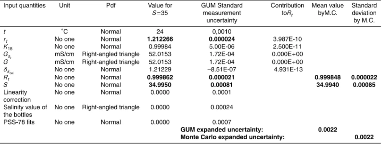
and the Monte Carlo methods. In order to realise reckonings according to the Monte Carlo method, the software Oracle Cristall Ball realise 11.1.1.1.000, has been used under a Microsoft Excel 2002. The Table 1 summarizes the parameters of the input quantities and the results. It appears that the biggest contribution to the uncertainty

15

onR_t comes from the temperature stability via r_t variations. The second contribution comes from the uncertainty on theK15 ratio.

Then, the uncertainty onS has been calculated using the relation of the PSS-78:

S =

5

X

j=0 ajR

j/2

t +

(t−15)

1+k(t₋15)

5

X

j=0 bjR

j/2

t (9)

where k, a_j and b_j are constants given for the calculation of salinity (Perkin et al.,

20

1980). This relation has two input variables: Rtand t. Rtdepends of tby the ratio rt.

The correlation coefficientrR_t,t can be calculated. At atmospheric pressure, forS=35,

r_R_t,t=0.55, forS=40,r_R_t,t=0.54, so that forS=10,r_R_t,t=0.97. The combined standard uncertaintyuc(S) ofS is then given by the relation:

u2_c(S)=

_∂S

∂R_t

2

u2_c(R_t)+

_∂S

∂t

2

u2_t +2r_R_t_,t ∂S ∂R_t

∂S

∂tuc(Rt)ut (10)

(8)

OSD

6, 2461–2485, 2009

calculations

M. Le Menn

Full Screen / Esc

where:

∂S ∂R_t =

_a

1

2R

−1/2

t +a2+

3a3

2 R

1/2

t +2a4Rt+

5a5

2 R

3/2

t

+ (t−15)

1+k(t−15)

×

_b

1

2 R

−1/2

t +b2+

3b3

2 R

1/2

t +2b4Rt+

5b5

2 R

3/2

t (11) and, ∂S ∂t = 1

[1+k(t−15)]2





5

X

j=0 bjR

j/2

t



 (12)

5

The Table 1 gives the values ofu_c(S) obtained with GUM computation (0.00081) and with Monte Carlo simulation (0.00085) for the salinity S=35. For S=10, the same computations give 0.00023 and 0.00025 and for S=40: 0.00099 and 0.0011. These calculations show that relation (10) can be simplified because the contribution of the first term is largely superior the contribution of the others, and it can be written:

10

uc(S)≈

∂S ∂Rt

uc(Rt) (13)

But, other uncertainties must be taken into account in the calculation of the uncertainty on salinity. At first, salinometers must be controlled at other standard salinities than 35, to correct for their linearity errors. These errors can be of 0.003 or more atS=2, as seen in calibration reports made by OSIL on Portasal salinometers (see Fig. 1).

15

Hardware corrections are difficult to realise because linearity can be un-constant in the range of measurement. Then, salinity values must be corrected by linear relations on different sub-ranges. These corrections have a standard uncertaintyu_l which is at least equal to the linear regression remainder or 0.0001.

At second, standard salinity bottles used for the calibration and the linearization can

20

(9)

OSD

6, 2461–2485, 2009

calculations

M. Le Menn

Title Page

Tables Figures

◭ ◮

Back Close

Full Screen / Esc

this uncertainty (usb) according to the GUM. The standard deviation of such a function

leads to expressu_sb as:usb=0.001/√3.

At third, PSS-78 relations fits have a standard deviation which is of 0.0007 at atmo-spheric pressure according to Perkin and Lewis (1980) and of 0.0015 if the pressure termR_pis different of 1. The pdf of this uncertainty (u_PSS) can be considered as being

5

Normal. In the case of salinometers,uPSS=0.0007.

u_l ,u_sb ,uPSS anduc(S) being independent variables,the expanded uncertaintyUS

on the salinity can be express as:

U_S =2

q

u_c(S)2₊_u2

l +u

2

sb+u

2

PSS (14)

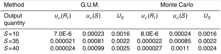
Table 1 gives the values ofUS computed with the GUM and the Monte Carlo methods

10

and it is the same whatever the method: U_S=0.0022 for S=35 for a Portasal sali-nometer. Table 2 gives the values obtained forS=10 and 40. It appears that the two methods give close results and that for 35 and 40 the expected accuracy of 0.002 can-not be respected. The main sources of errors are the stability of the bath temperature, the linearity of the salinometer, the salinity of the bottles of standard seawater and the

15

PSS-78 itself.

3 Uncertainties on reference conductivities calculations

Calibration of conductivity sensors needs the calculation of reference conductivities

Cref. When calibrations are made at atmospheric pressure,Cref is calculated with the

relation:

20

Cref=RtrtC(35,15,0) (15)

where rt is given by the relation (3) and Rt is obtained according to Fofonoff et al.

(1983), with a Newton–Raphson iteration and the formula:

R_tn+1=Rtn+(S−Sn)

_∂S

∂R_t

−1

(10)

OSD

6, 2461–2485, 2009

calculations

M. Le Menn

Title Page

Tables Figures

◭ ◮

Back Close

Full Screen / Esc

on condition to calculate (∂S/∂Rt) with the first part of the relation (11).

C(35,15,0) is a constant which value is much debated. According to Culkin and Smith (1980), C(35,15,0)=42.914 mS/cm and according to Poisson (1980),

C(35,15,0)=42.933 mS/cm. A recent study to be published by a BIPM working group (CCQM pilot study P111) has attributed the value 42.9104 mS/cm toC(35,15,0), after

5

inter-comparisons made by different metrology laboratories (Seitz et al., 2009). In fact, in the case of CTD conductivity sensors calibrations, it does no matter which value is used, provided that the same value be used during data reduction and reference con-ductivities computations. Most of recent instruments are referenced to 42.914, then, let us take this value in uncertainties calculations, C(35,15,0) being considered as

10

a constant.

The value of R_t obtained with the relation (16), depends essentially of S which is measured by a laboratory salinometer and rt depends of t. Then, we can write that

u_R_t=(∂R_t/∂S)u(S) andu_r_t=(∂r_t/∂t)u_t. But, the computation of numerical values ofR_t

andrtfor different temperatures between 0 and 40◦C, shows that the correlation

coef-15

ficientr_R_t_,r_t is not equal to zero. Forp=0 and S=35,r_R_t_,r_t=0.53, forS=40,r_R_t_,r_t=0.56 and forS=10,rRt,rt=0.964. Then, they can’t be considered as two independent vari-ables, and the combined uncertainty onCref is given by:

u_C_ref =C(35,15,0)

×

"

r2

t

_∂R

t

∂S

2

u2₍_S₎

+R2

t

_∂r

t

∂t

2

u2

t +R

_∂R

t

∂S

∂rt

∂t

u(S)u_tr_R_t_,r_t

#1/2

(17)

20

(∂S/∂R_t) can be calculated with the main part of the relation (11) andu(S)=U_S/2,U_S

being calculated with the relation (14).

(∂rt/∂t) is the polynomial of the relation (8), but in the relation (17)utis the

uncer-tainty on the reference temperatures measured during the calibration of the conductivity sensor. u_tdepends on the uncertainties of the calibration of the reference

thermome-25

(11)

OSD

6, 2461–2485, 2009

calculations

M. Le Menn

Title Page

Tables Figures

◭ ◮

Back Close

Full Screen / Esc

two calibrations, of its self-heating during the measurements and on the stability and uniformity of the calibration bath temperature.

In 2002, the BIPM has edited a guide (Fellmuth et al., 2002) about calibration un-certainties budgets of standard platinum reference thermometers (SPRT) to the fixed points of the ITS-90. It takes into account the calibration uncertainties of the fixed

5

points cells themselves, the realisation of the points, the self-heating errors and the repetability of the sensors but also, the non-unicities of the scale. This uncertainties budget can be applied to other kind of reference thermometers like Sea Bird Electron-ics SBE 35 which are used to calibrate CTD profilers at sea. In the best case, it leads to a combined standard uncertainty of 0.39 mK. This value is largely dependent of the

10

uncertainty of the temperature assigned to the reference cells, which is given by the pri-mary calibration laboratories. For example, a gallium melting point cell calibrated in UK with a UKAS certificate will have an expanded uncertainty of_±0.25 mK. The same cal-ibration made in France by the National Calcal-ibration Laboratory (LNE) under the same procedure, with a COFRAC certificate, will be given with an expanded uncertainty of

15

1.2 mK, which will give a combined uncertainty of 0.7 mK.

The drift of a reference thermometer between two annual calibrations can be equiv-alent to a standard uncertainty of 0.1 mK and the self-heating correction can lead to a standard uncertainty of 0.2 mK. The stability and the uniformity of the temperature of the calibration bath can be evaluated by the shifts and the standard deviations of series

20

of data measured at different places in the bath. It will express the reproducibility of measurements at all places in the bath. This reproducibility can be estimated, in the best case for seawater bath, to 0.3 mK in the range 0–40◦_C.

Then, the reference temperature combined uncertainty can be, in the best case, of:

ut=0.54 mK. With a COFRAC certificate on the fixed points cell: ut=0.80 mK.

25

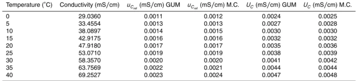
Table 3 shows values of uC_ref calculated for different temperatures, conductivities

(12)

OSD

6, 2461–2485, 2009

calculations

M. Le Menn

Title Page

Tables Figures

◭ ◮

Back Close

Full Screen / Esc

or superior to 0.002 mS/cm for high conductivity values. It appears also that the cross-term of the expression (17) can’t be neglected.

Conductivity sensors of CTD floats or profilers are linearized with polynomials before to be used at sea. Then, in order to know the uncertainty on the measured conduc-tivity, one must add to u_C_ref, the square sum of the polynomial residuals u_C_l and the

5

uncertainty on the CTD sensor readings which can be assessed by the repetability of the sensor measurementsuC_r. uC_ref, uC_l and uC_r being independent variables, the

expanded uncertaintyU_C on the conductivity values measured at sea, can be express as:

U_C =2qu2

Cref +u

2

Cl +u

2

Cr (18)

10

An estimate of the annual drifting of the sensor could be adds to this sum to have a real idea of the uncertainty on conductivity measurement. This source of errors has very variable amplitudes because it depends on the environment and the duration of measurements but also on the using of anti-fouling devices or on the regularity of the sensor cleaning. It varies from 0.001 mS/cm/year to several 0.01 mS/cm/year. In

15

order to illustrate this variation, Fig. 2 shows the statistics of 32 thermosalinographs SBE 21 calibrated yearly to the SHOM calibration laboratory since 2003, in the shame of the French operational oceanography project Coriolis which contributes to ARGO and GODAE experiences. This figure shows the drifts of conductivity cells submitted to strong environmental conditions.

20

So, in order to assess the value of U_C, we will just consider the initial uncertainty of the measurements. A usual value foru_C_l is 0.0002 mS/cm and we can take as an example the repetability of a Sea Bird Electronics SBE 4 conductivity cell, which can be considered as equivalent to their resolution or u_C_r=0.0004 mS/cm and it follows a Normal law.U_Chas been calculated with these values and the results are also given

25

(13)

OSD

6, 2461–2485, 2009

calculations

M. Le Menn

Title Page

Tables Figures

◭ ◮

Back Close

Full Screen / Esc

4 Uncertainties on salinities calculated from CTD sensors data

Salinity is calculated with relation (9) when data are measured up with CTD sensors, but pressure effect must be taken into account and in this case,Rtis obtain with:

Rt=

R rtRp

(19)

In this relation,r_t is given by the relation (3) and its uncertainty by the relation (8), in

5

whichutis the standard uncertainty on the temperatures measured by the CTD sensor.

Taking into account the elements given in the previous paragraph about temperature calibration and the quality of the CTD’s temperature sensors,u_t can be estimated to be equal to 0.001◦_C.

R is the ratio:

10

R= C(S, t, p)

C(35,15,0) (20)

C(S, t, p) is the conductivity measured by the conductivity sensor and which ex-panded uncertainty is given by the relation (18). C(35,15,0) is the constant which value has been discussed in the previous paragraph.C(35,15,0)=42.914 mS/cm and

uR=uC=UC/2, values ofUC being given in Table 3.

15

Rpis the coefficient for pressure effects correction. Rpis given by:

R_p=1+

pe1+e2p+e3p 2

1+d1t+d2t2+(d3+d4t)R

(21)

e1, e2, e3 et d1, d2, d3, d4 are constants which values are given in Perkin and Lewis

(1980). p and t are two independent quantities, but R, which is proportional to

C(S, t, p), is strongly correlated tot. The calculation of the correlation coefficientr_R,t,

(14)

OSD

6, 2461–2485, 2009

calculations

M. Le Menn

Title Page

Tables Figures

◭ ◮

Back Close

Full Screen / Esc

with the temperature – conductivity data of Table 3 gives r_R,t=0,9995. Let us take

rR,t≈1. In this case, the combined standard uncertainty onRp(uR_p) can be written:

u2

Rp =

∂Rp

∂p

!2

u2

p+

∂Rp

∂t ut+ ∂Rp

∂R uR

!2

(22)

The calculation of the sensitivity coefficients leads to write the final relation:

u_R_p =

5

e1+2e2p+3e3p 22

u2p+ Rp−1

2

(d1+2d2t+d4R)ut+(d3+d4t)uR

2 1/2

1+d1t+d2t2+(d3+d4t)R

(23)

It stays to find the value of u_p, the standard uncertainty on pressure measurements. Accuracy and precision of pressure sensors depend of their range of measurement. Pressure balances used to calibrate them, must be corrected to the normal gravity, of

10

the height difference with the sensor, of the thermal and pressure expansion of the piston and of the air – mass hydrostatic pressure difference. After that, the expanded uncertainty of a reference pressure given by a 8000 dbar balance is calculated by a relation of this kind:

UPref=0.12+0.00013p (dbar) (24)

15

If the repetability of a 6000 dbar sensor, and its electronics, is 0.2 dbar so that its residual temperature drift, thenup=0.53 dbar at 6000 or 0.34 dbar at 2000 dbar.

With those elements, it stays to write the expression of the standard combined uncer-tainty onRt, obtained with relation (19). Then, the GUM method applied to relation (19)

leads to write:

20

u_c(R_t)2 =

_∂R

t

∂R

2

u2_R + ∂Rt

∂R_p

!2

u2_R

p+

_∂R

t

∂r_t

2

u2_r_t +2∂Rt

∂R ∂Rt

(15)

OSD

6, 2461–2485, 2009

calculations

M. Le Menn

Full Screen / Esc

Interactive Discussion +2∂Rt

∂rt

∂R_t ∂Rp

ur_tuR_prr_t,R_p+2

∂R_t ∂R

∂R_t ∂rt

uRur_trR,r_t (25)

The development of the relation (25) gives:

u_c(R_t) =R_t uR R

2

+

u_R_p

R_p !2 + u r_t rt 2

−2u_RR u_R_p

R_prR,Rp+2

u_R_p

R_p ur_t

rt

r_r_t_,R_p

−2u_RR ur_t

rt

r_R,r_t

1/2

(26)

The correlation coe_fficients of the variables R, Rt and rt have been computed for

5

the salinities S=10, 35, 38 and 40, with the numerical values of t, C and p dis-played in Table 4. That gives: r_R,R_p=−0.44, rR,rt=0.998≈1 and rRp,rt=−0.50, and show that cross-terms can’t be neglected. More, neglecting these terms would leads to increase the uncertainty. For example, for t=2◦_C, _C

=33.038 mS/cm and

p=6000 dbar, u_c(R_t)=5_×10−4 and u_c(S)=0.0019, so that with the correlations terms,

10

u_c(R_t)=1.4_×10−5 and u_c(S)=0.0005! The uncertainties on practical salinity compu-tations take advantage of the ratio expression of R_t which reduces the effect of the uncertainties on each input variables.

With the correlation coefficients given previously, relation (26) can be simplified to give:

15

uc(Rt)=Rt

" _u

R

R −

ur_t

rt

2

+

u_R_p

R_p u_R_p

R_p +0.88 u_R

R −

ur_t

rt

!#1/2

(27)

(16)

OSD

6, 2461–2485, 2009

calculations

M. Le Menn

Title Page

Tables Figures

◭ ◮

Back Close

Full Screen / Esc

Then, in the case of CTD measurements, the expanded uncertainty on salinity com-putations can be assessed by the relation:

U_S =2

q

u_c(S)2₊_u2

PSS (28)

whereu_c(S) can be calculated with relations (13) and (26) or (27).

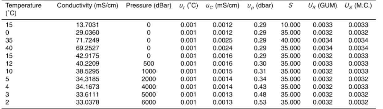
Table 4 shows the expanded uncertainties on practical salinities calculated from

re-5

lation (28) and with the Monte Carlo method. The two methods give equivalent results (U_S=0.0034 on average), which are superior of about 0.0014 to the 0.002 expected by the WOCE program.

More, this uncertainty assessment is valid only in areas where temperature and salin-ity gradients are low. When measurements are made in areas of strong temperature

10

and (or) salinity gradients, the major errors on practical salinity measurements come from the ability to align the response times of temperature and conductivity sensors, even when data are corrected with manufacturers correction algorithms, as shown by Mensah et al. (2009) recently. Errors up to 0.017, on average, still persist for some measurements in strong salinity gradients and increase as much the uncertainty on

15

practical salinity if they can’t be detected and corrected.

Lastly, one must not forget that practical salinity is only a way to approach the abso-lute salinity of seawater which is the real quantity to access thermodynamic properties of the ocean and ocean – atmosphere interactions. Therefore, non-electrolytes compo-nents are not detected by conductivity sensors and that leads an uncertainty of 0.16 ppt

20

even atS=35, as estimated by Jackett et al. (2006). Then, the expanded uncertainty of 0.0034 onS, as obtained with relation (28), can be considered as largely sufficient and even inconsiderable in the assessment of the absolute salinity.

5 Conclusions

The uncertainties of practical salinity calculations have been assessed by two

stan-25

(17)

OSD

6, 2461–2485, 2009

calculations

M. Le Menn

Title Page

Tables Figures

◭ ◮

Back Close

Full Screen / Esc

salinities obtained with laboratory salinometers and in the case of CTD measurements after laboratory calibration of conductivity cells. The two methods give coherent and very similar results. The 0.002 psu required initially by the WOCE program are hardly hold, even in the case of laboratory salinometers. But, in the error budget, the part due to the PSS-78 relations fits is sometimes as much significant as the instruments one’s.

5

This is particularly the case with CTD measurements where correlations between the

R_t variables contribute to decrease largely the uncertainty on S, even when the ex-panded uncertainties on conductivity cells calibrations are largely up of 0.002 mS/cm. The relations given in this publication and obtained with the normalized GUM method, allow a real analysis of the uncertainties sources and they can be used in a general way

10

to assess the uncertainty on conductivity cells calibrations or practical salinity calcula-tion made with data from instruments having different specifications than the examples taken in Tables 1 to 4.

Appendix A

15

PSS 78 algorithm as defined in Fofonoffet al. (1983)

pis expressed in dbar,tin◦C andCin S/m

a1=0.0080,a2=−0.1692,a3=25.3851,a4=14.0941,a5=−7.0261,a6=2.7081 b₁=0.0005,b₂=−0.0056,b3=−0.0066,b4=−0.0375,b5=0.0636,b6=−0.0144

c1=0.676697,c2=2.00564E−2,c3=1.104259E−4,c4=−6.9698E−7,c5=1.0031E−9 20

d1=3.426E−2,d2=4.464E−4,d3=0.4215,d4=−3.107E−3 e1=2.070E−5,e2=−6.370E−10,e3=3.989E−15

Probe:

R=C/4.2914

R1=c1+(c2+(c3+(c4+c5×t)×t)×t)×t 25

(18)

OSD

6, 2461–2485, 2009

calculations

M. Le Menn

Title Page

Tables Figures

◭ ◮

Back Close

Full Screen / Esc

References

Bacon, S., Culkin, F., Higgs, N., and Ridout, P.: IAPSO Standard Seawater: definition of the uncertainty in the calibration procedure and stability of recent batches, J. Atmos. Ocean. Tech., 24, 1785–1799, 2007.

BIPM: Evaluation of measurement data – Supplement 1 to the Guide to the expression of

5

uncertainty in measurement – Propagation of distributions using a Monte Carlo method, Joint Committee for Guides in Metrology, YYY:2006, 60 pp., 2006.

BIPM: Evaluation of measurement data – Guide to the expression of uncertainty in measure-ment, JCGM 100:2008, GUM 1995 with minor corrections, 2008.

Culkin, F. and Smith, N.: Determination of the concentration of potassium chloride solution

10

having the same electrical conductivity, at 15◦_{C and infinite frequency, as standard seawater} of salinity 35000‰, (Chlorinity 19.37394%), IEEE J. Ocean. Eng., 5(1), 22–23, 1980. Culkin, F. and Ridout, P. S.: Stability of IAPSO Standard Seawater, J. Atmos. Ocean. Tech., 15,

1072–1075, 1997.

Fellmuth, B., Fisher, J., and Tegeler, E.: Uncertainty budgets for characteristics of SPRTs

cali-15

brated according to the ITS-90, BIPM, CCT/01–02, 2002.

Fofono_ff, N. P. and Millard, R. C.: Algorithms for computation of fundamental properties of seawater, Unesco Technical Paper in Marine Science, 44, 53 pp., 1983.

Jackett, D. R. and McDougall, T. J.: Algorithms for density, potential temperature, conservative temperature and the freezing temperature of seawater, J. Atmos. Ocean. Tech., 23, 1709–

20

1728, 2006.

Kawano, T., Aoyama, M., and Takatsuki, M.: Inconsistency in the conductivity of standard potassium chloride solutions made from different high-quality reagents, Deep-Sea Res. I, 52, 389–396, 2005.

Mensah, V., Le Menn, M., and Morel, Y.: Thermal mass correction for the evaluation of

salin-25

ity, J. Atmos. Ocean. Tech., 26(3), 665–672, 2009.

Perkin, R. G. and Lewis, E. L.: The practical salinity scale 1978: Fitting the data, IEEE J. Ocean. Eng., 5(1), 9–16, 1980.

Poisson, A.: Conductivity/Salinity/Temperature relationship of diluted and concentrated stan-dard seawater, IEEE J. Oceanic Eng., 5(1), 41–50, 1980.

30

(19)

OSD

6, 2461–2485, 2009

calculations

M. Le Menn

Title Page

Tables Figures

◭ ◮

Back Close

Full Screen / Esc

Seitz, S., Spitzer, P., and Brown, R. J. C.: Consistency of practical salinity measurements traceable to primary conductivity standards: Euromet project 918, Accred. Qual. Assur., 13, 601–605, 2008.

Seitz, S. and Spitzer, P.: Establishment of SI traceability of Practical Salinity in Oceanographic Research, session 14, 14th Int. Congr. Metrol., Paris, June 2009.

5

(20)

OSD

6, 2461–2485, 2009

calculations

M. Le Menn

Title Page

Tables Figures

◭ ◮

Back Close

Full Screen / Esc

Interactive Discussion Table 1. Parameters of the input quantities used to compute the expanded uncertainty of

Guildline Portasal salinometer forS=35, by the GUM and the Monte Carlo (M.C.) methods.

Input quantities Unit Pdf Value for GUM Standard Contribution Mean value Standard

S=35 measurement toRt byM.C. deviation uncertainty by M.C.

t ◦_C _Normal ₂₄ _0,0010

rt No one Normal 1.212266 0.000024 3.987E-10

K15 No one Normal 0.99984 5.00E-06 2.500E-11 Gst mS/cm Right-angled triangle 52.0153 1.72E-04 0.000E+00

G mS/cm Right-angled triangle 52.0153 1.72E-04 0.000E+00

δk_cell No one Normal 1.21229 –8.51E-07 4.931E-13

Rt No one Normal 0.999862 0.000021 0.999848 0.000022

S No one Normal 34.9950 0.00081 34.9940 0.00085

Linearity correction

No one Normal 0.0000 0.0001

Salinity value of the bottles

No one Right-angled triangle 0.0000 0.00024

PSS-78 fits No one Normal 0.0000 0.0007

GUM expanded uncertainty: 0.0022

(21)

OSD

6, 2461–2485, 2009

calculations

M. Le Menn

Title Page

Tables Figures

◭ ◮

Back Close

Full Screen / Esc

Interactive Discussion Table 2.standard uncertainties ofR_t andS, and expanded uncertainty on the corrected value

of S, calculated by the two methods for three di_fferent salinities. These values don’t take into account possible long term variations in KCl standard solutions used to adjust standard seawater bottles.

Method G.U.M. Monte Carlo

Output quantity

uc(Rt) uc(S) US uc(Rt) uc(S) US

S=10 7.0E-6 0.00023 0.0016 8.0E-6 0.00024 0.0016

S=35 0.000021 0.00081 0.0022 0.000022 0.00085 0.0022

(22)

OSD

6, 2461–2485, 2009

calculations

M. Le Menn

Title Page

Tables Figures

◭ ◮

Back Close

Full Screen / Esc

Interactive Discussion Table 3. Standard combined uncertainties on reference conductivities (u_C

ref), computed for

different values of temperature, conductivity and forS=35, and expanded uncertainty on con-ductivity values measured with linearized sensors (U_C). U_Candu_C

refhave been assessed with

the GUM and the Monte Carlo Method (M.C.).

Temperature (◦_C) _{Conductivity (mS}_/_cm) _uC

ref(mS/cm) GUM uCref(mS/cm) M.C. UC(mS/cm) GUM UC(mS/cm) M.C.

0 29.0360 0.0011 0.0012 0.0024 0.0025

5 33.4554 0.0013 0.0013 0.0027 0.0028

(23)

OSD

6, 2461–2485, 2009

calculations

M. Le Menn

Title Page

Tables Figures

◭ ◮

Back Close

Full Screen / Esc

Interactive Discussion Table 4.Expanded combined uncertainties on salinity, computed with representative values of

temperature, conductivity and pressure and their combined standard uncertainties. Conduc-tivity combined standard uncertainties u_C correspond to the values found in Table 3 and for temperature, the standard uncertainty correspond to the best case whenu_t=0.001◦_{C. Idem for}

u_p.

Temperature (◦_C)

Conductivity (mS/cm) Pressure (dBar) ut(◦_C) _uC_(mS/cm) _up_(dbar) _S _US_(GUM) _US_(M.C.)

(24)

OSD

6, 2461–2485, 2009

calculations

M. Le Menn

Title Page

Tables Figures

◭ ◮

Back Close

Full Screen / Esc

Interactive Discussion -0 ,0 0 6 0

-0 ,0 0 5 0 -0 ,0 0 4 0 -0 ,0 0 3 0 -0 ,0 0 2 0 -0 ,0 0 1 0 0 ,0 0 0 0 0 ,0 0 1 0

1 0 3 0 3 5 38

Reference salinity

S

a

li

n

it

y

e

r

o

r

P o rt asal n °1

P o rt asal n °2

P o rt asal n °3

(25)

OSD

6, 2461–2485, 2009

calculations

M. Le Menn

Title Page

Tables Figures

◭ ◮

Back Close

Full Screen / Esc

0 5 10 15 20 25 30

%

0.00 to 0.01

0.01 to 0.02

0.02 to 0.03

0.03 to 0.04

0.04 to 0.05

0.05 to 0.06

0.06 to 0.07

> 0.07

mS/cm