www.atmos-chem-phys.net/14/3573/2014/ doi:10.5194/acp-14-3573-2014
© Author(s) 2014. CC Attribution 3.0 License.
Atmospheric
Chemistry
and Physics
Atmospheric parameters in a subtropical cloud regime transition
derived by AIRS and MODIS: observed statistical variability
compared to ERA-Interim
M. M. Schreier1,2, B. H. Kahn2, K. Sušelj1,2, J. Karlsson2,3, S. C. Ou1, Q. Yue1,2, and S. L. Nasiri4
1Joint Institute for Regional Earth System Science and Engineering, University of California – Los Angeles, Los Angeles, CA, USA
2Jet Propulsion Laboratory, California Institute of Technology, Pasadena, CA, USA
3Department of Meteorology and Bolin Centre of Climate Research, Stockholm University, Sweden 4Department of Atmospheric Sciences, Texas A&M University, College Station, TX, USA
Correspondence to:M. M. Schreier ([email protected])
Received: 18 July 2013 – Published in Atmos. Chem. Phys. Discuss.: 12 September 2013 Revised: 14 February 2014 – Accepted: 18 February 2014 – Published: 9 April 2014
Abstract.Cloud occurrence, microphysical and optical
prop-erties, and atmospheric profiles within a subtropical cloud regime transition in the northeastern Pacific Ocean are ob-tained from a synergistic combination of the Atmospheric Infrared Sounder (AIRS) and the MODerate resolution Imag-ing Spectroradiometer (MODIS). The observed cloud param-eters and atmospheric thermodynamic profile retrievals are binned by cloud type and analyzed based on their proba-bility density functions (PDFs). Comparison of the PDFs to data from the European Centre for Medium Range Weather Forecasting reanalysis (ERA-Interim) shows a strong differ-ence in the occurrdiffer-ence of the different cloud types compared to clear sky. An increasing non-Gaussian behavior is ob-served in cloud optical thickness (τc), effective radius (re)
and cloud-top temperature (Tc)distributions from
stratocu-mulus to trade custratocu-mulus, while decreasing values of lower-tropospheric stability are seen. However, variations in the mean, width and shape of the distributions are found. The AIRS potential temperature (θ )and water vapor (q) profiles
in the presence of varying marine boundary layer (MBL) cloud types show overall similarities to the ERA-Interim in the mean profiles, but differences arise in the higher moments at some altitudes. The differences between the PDFs from AIRS+MODIS and ERA-Interim make it possible to pin-point systematic errors in both systems and help to under-stand joint PDFs of cloud properties and coincident thermo-dynamic profiles from satellite observations.
1 Introduction
Earth’s cloud types are highly variable in both their fre-quency of occurrence and optical properties, and therefore have strong relevance to climate sensitivity (see, e.g., Cess et al., 1989, 1996; Bony and DuFresne, 2005; Wyant et al., 2006; Vial et al., 2013; or IPCC, 2007). The spatial and tem-poral variation in cloud types are controlled to a significant degree by the large-scale atmospheric dynamic circulation and thermodynamic structures (Stephens, 2005; Bony and Dufresne, 2005; Su et al., 2008) in combination with vari-ations of water vapor (Stevens, 2005). However, on a smaller scale, the water vapor within clear-sky conditions can be influenced by adjacent clouds (Stevens, 2005), resulting in variations of water vapor. Quantifying the variations of po-tential temperature (θ )and water vapor (q) profiles within
each cloud type is therefore essential for understanding the spatial and temporal variability of clouds in a present and fu-ture climate. There is also an increased interest in the analysis of joint probability distribution functions (PDFs) of parame-ters such asθand total water contentqt, which could be used to develop subgrid-scale climate model parameterizations to represent variability within a general circulation model (GCM) grid. Based on early ideas (Sommeria and Dear-dorff, 1977; Cuijpers and Bechthold, 1995), the importance of cloud-dependent statistics for θ andq has been pointed
Quaas (2012) and Randall (2013). Recent studies such as those by Guo et al. (2010) and Bogenschutz et al. (2013) have been various attempts to implement and improve such schemes in climate models.
Satellite data and reanalysis data might be a helpful tool in the investigating of PDFs of cloud regimes in remote re-gions. A particular remote area of cloud regime transition is the stratocumulus (Sc) to trade cumulus (trade Cu) transition (Hartmann et al., 1992; Teixeira et al., 2011). This region is thought to be a significant contributor to uncertainty in the magnitude of climate sensitivity in global climate models and it is still a matter of debate as to which portion of cloudi-ness within this area dominates the uncertainty in climate sensitivity (Cess et al., 1989; Wood and Bretherton, 2006; Medeiros et al., 2008). The radiative feedbacks of the vari-ous types of marine boundary layer (MBL) clouds show large variations between different GCM simulations (Williams and Webb, 2009). Therefore, detailed observations of cloud prop-erties, thermodynamic profiles and spectral radiances includ-ing their means, variances and higher order statistical mo-ments are necessary to establish meaningful constraints for climate modeling efforts (Weber et al., 2011).
In situ observations are sparse in this area (Albrecht et al., 1995; Norris, 1998; Price and Wood, 2002; Tompkins, 2003), or based on limited time periods such as the Second Dy-namics and Chemistry of Marine Stratocumulus field study (DYCOMS-II; Stevens et al., 2003) or the Marine ARM GPCI Investigation of Clouds (MAGIC; Lewis al., 2012). Therefore, the main source ofθ andq information is from
reanalysis data such as ERA-Interim. Our aim is to validate information from these reanalysis profiles with contempo-rary A-train satellite data. Furthermore, we are interested in whether the satellite data provide additional quantitative in-formation regarding the higher moments of the PDFs that the reanalysis may be lacking. There are systematic biases in the ERA-Interim low-latitude cloud regimes that have been pre-viously discussed (Dee et al., 2011). In particular, the ver-sion of the Integrated Forecast System (IFS) most similar to that used in ERA-Interim (CY31R1) overestimates the pop-ulation of trade cumulus while underestimating the cloud fraction, and has a high-altitude bias relative to the Cloud-Aerosol Lidar and Infrared Pathfinder Satellite Observation (CALIPSO) lidar (Ahlgrimm and Köhler, 2010).
Infrared and microwave satellite sounders are capable of continuously observing the global oceans on a daily basis, albeit with coarser spatial and temporal resolution, as well as reduced precision and accuracy, compared to in situ ob-servations. An example of these satellite sounders is the At-mospheric Infrared Sounder (AIRS)/Advanced Microwave Sounding Unit (AMSU) (Aumann et al., 2003), onboard the Earth Observing System (EOS) Aqua satellite, which has been operational since September 2002. AIRS/AMSU is an advanced sounding suite designed to retrieve temperature and water vapor profiles in clear and cloudy skies for cloud amounts up to and exceeding 70 % (Susskind et al., 2006;
Yue et al., 2011). The use of infrared retrievals in the lower troposphere remains a challenge due to the decreasing in-formation content and the difficulty in detecting low-cloud contamination. However, recent investigations (e.g., Kahn et al., 2011b; Martins et al., 2011, Yue et al., 2013) have shown that AIRS/AMSU is capable of observing coarse-layer ther-modynamic structures in the planetary boundary layer.
Together with the MODerate resolution Imaging Spec-troradiometer (MODIS; Barnes et al., 1998), also onboard EOS Aqua, it is possible to observe and estimate clouds with high spatial resolution (∼1–5 km, depending on the de-rived geophysical product) yielding sub-footprint informa-tion about cloud variability within the AIRS/AMSU field of view (FOV). Combining the information obtained from the two sensors has resulted in advances in cross-sensor radi-ance calibration (Tobin et al., 2006; Schreier et al., 2010), synergistic multi-sensor cloud property retrievals (Li et al. 2004a, b) and cloud phase characterization (Kahn et al., 2011a). It is also a useful source of information for radia-tive transfer calculations under cloudy conditions (Ou et al., 2013) and offers a promising basis for improvements in ther-modynamic profile sounding (e.g., Maddy et al., 2011).
The synergistic use of AIRS and MODIS offers a unique opportunity to characterize simultaneous PDFs ofθ,q and
cloud properties – including optical thickness (τc), effective
radius (re)and cloud-top temperature (Tc)– and quantify
re-lationships between these variables as a function of cloud type. In this study, we compare similarly derived PDFs from satellite data and the ERA-Interim reanalysis that are orga-nized by cloud type.
The coarse horizontal resolution of AIRS/AMSU is a fun-damental weakness. The remote sensing data (∼45 km) are only a factor of ∼ 2 higher than ERA-Interim resolution (∼80 km). While it is impossible to resolve very small scale features that will be effectively smeared over the 45 km field of regard, the reanalysis is also subject to the assumptions imposed by subgrid-scale parameterizations, for which the satellite data are not subject to. Thus, there is value in com-paring the two data sets. In this work, we examine whether the remote sensing observations ofθ,q and cloud property
PDFs are comparable to current state-of-the-art reanalysis data, especially in the case of the stratocumulus (Sc) to trade cumulus (trade Cu) transition. The level 2 satellite products are compared to identical PDFs obtained from the ERA-Interim reanalysis to quantify similarities and differences de-pending on cloud type.
2 Methodology
2.1 AIRS and MODIS observations
The EOS Aqua platform has a polar Sun-synchronous orbit with an equatorial local crossing time of 01:30 (descending) and 13:30 (ascending). AIRS is a grating spectrometer with a spectral resolution ofν/1ν ≈1200, a total of 2378 chan-nels in the range of 3.7–15.4 µm with a few spectral gaps, and well-calibrated level 1B radiances (Overoye, 1999). The AIRS FOV is approximately 1.1◦, resulting in a footprint size of 13.5 km at nadir view. There are 90 cross-track scan an-gles with the highest at±48.95◦, yielding a swath width of approximately 1650 km. AIRS is co-registered with AMSU (Lambrigtsen and Lee, 2003), and the combination is used to retrieveT,qand numerous other surface and atmospheric
parameters. Geophysical retrievals are obtained in clear sky and broken cloud cover using a cloud-clearing methodology (Susskind et al., 2003).
The MODIS instrument is a spectrometer based on a spec-tral filter aperture with 36 channels in the range of 0.4–14 µm and bandwidths of 0.01–0.5 µm, depending on the channel, and scans up to±55◦off nadir view. The pixel size depends on the channel and varies from 0.25–1.0 km at nadir. At 1 km resolution, there are 1354 cross-track pixels resulting in a swath width of approximately 2330 km. Several MODIS al-gorithms are designed to obtain a wide variety of land, ocean and ice surface characteristics, as well as atmospheric and oceanic geophysical properties that include numerous cloud and aerosol parameters. In this work, we use collection 5 cloud products, including the cloud mask (Ackerman et al., 2008; Frey et al., 2008), effective radius (re) and optical
thickness (τc)(Platnick et al., 2003), and cloud-top
tempera-ture (Tc)(Menzel et al., 2006).
The MODIS pixels are accurately collocated within the AIRS FOV using the AIRS spatial response functions ob-tained from prelaunch calibration activities (Schreier et al., 2010). Since AIRS and MODIS have FOV sizes of 1.1◦and 0.08◦ at nadir, respectively, this yields approximately 200 1 km pixels of MODIS within a given AIRS FOV. Using this collocation technique, the importance of each MODIS pixel can be weighted depending on its location within the AIRS spatial response function (Nasiri et al., 2011).
2.2 ERA-Interim reanalysis
The ERA-Interim reanalysis is used as a comparison stan-dard to the satellite observations. The reanalysis is an “in-terim” following ERA-40 (Uppala, et al., 2005), a meteoro-logical reanalysis that uses a wide variety of observations that include synoptic weather information, radiosondes, satellite data and model forecast data produced by the European Cen-tre for Medium-Range Weather Forecasts (ECMWF). The forecast model is the ECMWF Integrated Forecast System (IFS). While satellite data are used in the reanalysis,
pri-marily clear-sky AIRS or High Infrared Radiometer Sounder (HIRS) radiances are used; for more details see Dee et al. (2011). The reanalysis spatial resolution is based on a T255 truncation scheme, resulting in ∼79 km grid spacing on a reduced Gaussian grid, making it somewhat larger than the AIRS/AMSU footprint at nadir. The time steps of calcu-lation are 30 min, with an output frequency of 6 h. Cloud-top parameters (Tc,re,τc and cloud cover) from ERA-Interim were obtained in a manner that mimics the satellite observa-tions and is consistent with the parameterizaobserva-tions in ERA-Interim. First, the re and τc are calculated on each of the ERA-Interim levels using the same formulations as in reanal-ysis model parameterization (see IFS documentation, 2007); that is, thereis parameterized as a linear function of height and equals 10 µm at the surface and 45 µm at the top of the at-mosphere (which is taken to be 20 km). The optical thickness is parameterized as a function of the liquid water amount in a vertical level (ULWP)andreas
τc(z)=3 2
ULWP
re .
As our focus is mainly on boundary layer clouds, we con-sider only the liquid clouds. The cloud-top parameters (as one value per pixel) are then calculated by integration in the vertical as would be seen from space assuming maximum cloud overlap.
2.3 The stratocumulus to trade cumulus transition
Our examination is restricted to the northeastern Pacific Ocean between 0 and 40◦N latitude and between 125 and 175◦W longitude. A persistent stratocumulus to trade cumu-lus transition is bordered by deep convection in the tropics and midlatitude baroclinic systems. The highest frequency of stratocumulus occurs from June to September (Klein and Hartmann, 1993). The AIRS and MODIS instruments have provided daily and global data since late 2002. To investigate a reasonable subset of data and minimize interannual varia-tions, we focus on all available days in all 10 Julys from 2003 to 2012 for a total of 310 days.
Fig. 1.Shown is the primary region of interest in the northeastern Pacific Ocean along the GPCI transect (white boxes; Karlsson et al., 2010; Teixeira et al., 2011). The colored background is the mean low-cloud amount according to ISCCP (Rossow and Schiffer, 1999) for a July composite from 2003 to 2010. The overlay is a snapshot image from the 0.65 µm channel of MODIS from 1 July 2007.
is performed on the pixel scale within these boxes, with no averaging among the boxes.
The GPCI transect contains a broad range of cloud types. The main three MBL cloud types are namely stratocumulus (Sc), transition cumulus (trans Cu) and trade cumulus (trade Cu). The parameter that differentiates between these three broad MBL cloud categories is the cloud fraction, defined here as the percentage of cloudy pixels within a unit area. There is no precise definition of the spatial scale that ap-plies to cloud coverage as a discriminant for these three cloud types. The MODIS pixel-scale variability within the AIRS FOV was used to determine cloud fraction and the resulting MBL cloud type. In addition to the three categories of MBL cloud types, three additional categories for high clouds, mid-level clouds and clear sky are included, but no further sub-classification is attempted herein. The definition of each cat-egory is based on the MODIS cloud mask “confident cloud” and “probably cloud” categories and cloud-top pressure. The flag probably cloud was weighted with 50 % cloudy for con-sistency, but changes in this weighting do not affect the re-sults due to the low frequency of occurrence of this flag in the data sets. The definition of the cloud type within each AIRS FOV is as follows:
– trade Cu: cloud fraction < 30 % below 680 hPa, cloud
fraction < 1 % for above 680 hPa pressure level;
– trans Cu: cloud fraction 30–90 % below 680 hPa, cloud
fraction < 1 % for clouds above 680 hPa pressure level;
– Sc: cloud fraction > 90 % below 680 hPa, cloud
frac-tion < 1 % for clouds above 680 hPa pressure level;
– high clouds (high cld): cloud fraction > 90 % for
clouds above 440 hPa pressure level;
– mid-level clouds (mid cld): cloud fraction > 90 % for
clouds between 440–680 hPa;
– clear sky (clr): cloud fraction=0 %.
Only homogeneous FOVs (cloud fraction > 90 %) are used in the case of mid-level and high clouds to reduce the number of complicated cloud configurations in the study. For clear sky, only the clearest scenes (cloud fraction=0 %) are retained. Due to the cloud detection limits of MODIS (Ackerman et al., 2008), it is likely that some thin cirrus as well as subpixel-scale MBL clouds not detected by the MODIS cloud mask are contained in low-cloud or clear-sky scenes, or that some low clouds were classified as mid-level clouds. However, ad-justments in these definitions do not lead to any apprecia-ble changes in the statistics that follow. Another drawback of polar-orbiting satellites that must be considered is the in-stantaneous observation at 13:30 LT. The time dependence of the relationship between cloud coverage,θ andq cannot be
taken into account by daily snapshots at a fixed local time. The sample size of all profiles in this area exceed 1 800 000 for AIRS/MODIS. Around 55 % of them (1 000 000) fell into the defined cloud categories. Cloud properties were only re-tained when MODIS retrievals were successful within the AIRS footprint, reducing the total sample size to approxi-mately 980 000 data points. The AIRS/AMSU sounding suite encounters cloud-type-dependent sampling rates that may impact the “representativeness” ofθ andq statistics within
each cloud regime. Only “good” quality profiles are retained; the AIRS “PGood” flag is used to indicate a good retrieval to the ocean surface. Yue et al. (2011) used CloudSat and CALIPSO to quantify the sampling rate by cloud type. AIRS has sampling rates of 80–90 % in areas of trade Cu, and as much as 20–40 % within Sc regimes. In this study, approx-imately 900 000 profiles with successful retrievals are ob-tained for the 310-day period. Approximately 27 % of the data are found in trade Cu, 26 % in trans Cu, 20 % in Sc, 18 % in high clouds, 5 % in mid-level clouds and 4 % in clear sky.
2.4 Cloud-type statistics of thermodynamic profiles and cloud parameters
AIRS retrievals ofθandq, as well as MODIS cloud retrievals
of effective radius, cloud optical thickness and cloud-top height (re,τc, andTc), are quantified and sorted by the
afore-mentioned cloud types, and the same procedure is followed for ERA-Interim. To quantify differences between the differ-ent cloud types, statistics of each geophysical parameter are calculated separately for each cloud type and then compared to each other. Given a group of thermodynamic profiles and cloud parameters, the mean, standard deviation, skewness and kurtosis are calculated. To take into account the influence of time variability, we show, for each data set and cloud type, two types of profiles in these statistics: first, the average from daily “snapshots” for the 310-day period, and second, the to-tal average of all profiles from all 310 days. This is also done for the higher moments. The second moment (standard devia-tion) provides information about the variation from the mean. Skewness and kurtosis, the third and fourth moment, provide information about the shape of the distribution function. The skewness helps to identify asymmetry and side tails, whereas the kurtosis identifies the strength of the “peakedness” of the distribution. In the case ofθandq, the statistics are
calcu-lated individually for each vertical layer. This approach was taken to preserve height-dependent behavior in the PDFs. For the cloud parameters, the moments ofre,τcandTcare calcu-lated for each cloud type. The interpretations assume a single mode that neglects bimodality. This is a simplified assump-tion, as bimodality is possible in tropical water vapor (Zhang et al., 2006) and in non-steady-state cases (Sukhutame and Young, 2010), which could have an influence on skewness and kurtosis ofqfor trade Cu and high clouds. However, the
analysis of randomly selected layers ofθ andq for the
dif-ferent cloud types did not reveal any bimodal distributions in our data set and the simplified unimodal assumption is used for all calculations.
AIRS and MODIS are not the only instruments of rele-vance in the A-train for the quantification of the statistical state of MBL clouds in the GPCI cross section. However, the wide instrument swaths (AIRS: 1600 km, MODIS: 2330 km) facilitate the robust calculation of daily instantaneous spa-tial statistics. The active sensors with a narrow surface track (CloudSat and CALIPSO) do not sample in swaths and thus only the synergy of AIRS and MODIS is emphasized herein.
3 Results
Here we describe the observational and model-derived pa-rameters and their statistical moments. This includes the cloud-type-dependent PDFs ofre,τc andTc from MODIS, and the lower-tropospheric stability (LTS), θ and q from
AIRS.
3.1 Cloud parameters
Figure 2 shows the annual mean evolution of relative oc-currence and frequency distribution of cloud fraction of the defined types of clouds. The occurrence (panel a) for AIRS/MODIS and (panel b) for ERA-Interim is normal-ized relative to clear sky: 100 % translates as the same oc-currence of the cloud type as clear-sky ococ-currence for this month, whereas 200 or 300 % translate as 2 or 3 times more occurrence of this type than clear sky. We are using each July month separately and an average over all 10 July months (right of black line). On average, ERA-Interim shows a higher occurrence of low marine cloud types than observa-tions. In ERA-Interim, Sc occurs on average 9 times more often than clear sky, whereas the observations show a fac-tor of 6 difference. Similar differences are seen for trans Cu (ERA-Interim ∼11, AIRS/MODIS ∼7) and trade Cu (ERA-Interim∼9.6, AIRS/MODIS ∼7.5). However, mid-level clouds (ERA-Interim∼2.3, AIRS/MODIS∼2.4) and high clouds (ERA-Interim ∼6.6, AIRS/MODIS ∼6.2) are remarkably similar. There is also a substantial variation from year to year, with a strong peak in 2005 and 2010 for ERA-Interim and AIRS/MODIS in all cloud types. A detailed in-vestigation of seasonal variations is beyond the scope of this article and warrants further investigation.
The PDFs of cloud fraction are shown in the panels c and d of Fig. 2. The frequency of Sc cloud amount is weighted more heavily to near 100 % in MODIS compared to ERA-Interim. For trade Cu in AIRS/MODIS, the maximum fre-quencies are weighted near the bottom (0 %) of their respec-tive ranges, with a minimum around 30 % cloud fraction. In contrast, ERA-Interim shows a peak frequency of occurrence around 30 % cloud fraction, near the cut-off value for the definition of trade Cu and trans Cu. Thus, ERA-Interim is producing a higher occurrence frequency of low clouds than observations, but with a lower magnitude of cloud fraction compared to the observations. The limited spatial resolution (250 m to 1 km) of MODIS may somewhat overestimate the trade Cu population in comparison to trans Cu or Sc (Zhao and Di Girolamo, 2006).
Fig. 2.Annual and average occurrence of cloud types relative to clear sky (panelsaandb) and cloud fraction (panelscandd) for the entire 310-day data set. The left column is for the AIRS/MODIS observations, and the right is for ERA-Interim.
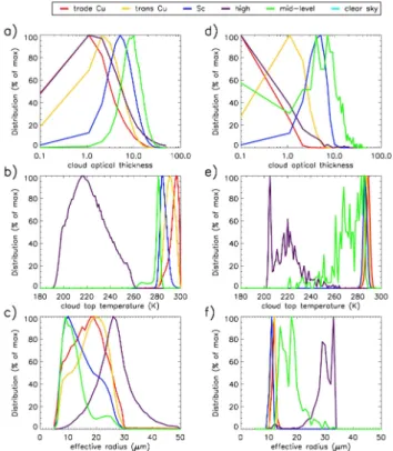
to report much lower occurrences of optically thin trade Cu compared to ERA-Interim (Fig. 2, panel d). The MODIS and ERA-Interim differences in the distribution of liquid water for trade and trans Cu suggests, in combination with the in-formation of occurrence and cloud coverage from the para-graph before, a biased distribution of cloud liquid water and cloud coverage within ERA-Interim compared to the obser-vations.
There are also several notable features in the Tc data (Fig. 3, panels b and e). The meanTc increases from Sc to trade Cu in both data sets. WhileTcincreases from 286.1 K in Sc to 294.4 K within trade Cu in MODIS, ERA-Interim only shows an increase from 286.7 to 289.1 K. This is consistent with expectations that trade Cu are found in lower latitudes over warm ocean surfaces compared to Sc. The overestima-tion ofTc from MODIS is consistent with a warmTc bias observed in MODIS partly cloudy pixels (Marchand et al., 2010). The large negative skewness observed inTcfor trade Cu is seen in both MODIS and ERA-Interim and is consistent with a small population of trade Cu skewed towards higher and colder altitudes capped by a weak trade wind inversion, and a large population at lower and warmer altitudes. In Sc and trans Cu, the distributions ofTcare nearly Gaussian, ex-cept for elevated kurtosis of Sc in ERA-Interim.
The mean re shows a substantial increase from Sc (12.3 µm) to trade Cu (17.7 µm) in the MODIS data. The ERA-Interim data show only a weak increase from 11.3 to 12.3 µm. The larger re may be a result of overestimation of droplet radii in the MODIS cloud retrieval (King et al., 2013). However, it is consistent with the occurrence of larger droplets from stronger updrafts and light precipitation and/or drizzle forre larger than 15 µm (Gerber, 1996; Masunaga et al., 2002) and is more realistic than ERA-Interim. For
Fig. 3.Cloud-type distributions ofτc(panelsaandd),Tc(panelsb ande) andre(panelscandf) for the entire 310-day data set. The left column is for the AIRS/MODIS observations, and the right is for ERA-Interim.
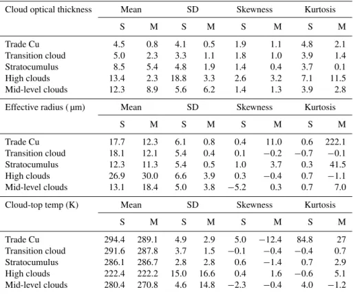
Table 1.Mean, standard deviation, skewness and kurtosis of MODIS-derived (“S” for satellite columns) and ERA-Interim-derived (“M” for model columns) cloud parameters (τc,re,Tc).
Cloud optical thickness Mean SD Skewness Kurtosis
S M S M S M S M
Trade Cu 4.5 0.8 4.1 0.5 1.9 1.1 4.8 2.1
Transition cloud 5.0 2.3 3.3 1.1 1.8 1.0 3.9 1.4
Stratocumulus 8.5 5.4 4.8 1.9 1.4 0.4 3.7 0.1
High clouds 13.4 2.3 18.8 3.3 2.6 3.2 7.1 11.5
Mid-level clouds 12.3 8.9 5.6 6.2 1.4 1.3 3.9 2.8
Effective radius ( µm) Mean SD Skewness Kurtosis
S M S M S M S M
Trade Cu 17.7 12.3 6.1 0.8 0.4 11.0 0.6 222.1
Transition cloud 18.1 12.1 5.4 0.4 0.1 −0.2 −0.7 −0.1
Stratocumulus 12.3 11.3 5.4 0.5 1.0 3.7 0.3 41.5
High clouds 26.9 30.0 6.6 3.9 0.3 −0.4 0.7 −1.1
Mid-level clouds 13.1 18.4 5.0 3.8 −5.2 0.3 0.7 7.0
Cloud-top temp (K) Mean SD Skewness Kurtosis
S M S M S M S M
Trade Cu 294.4 289.1 4.9 2.9 5.0 −12.4 84.8 27
Transition cloud 291.6 287.8 3.7 1.5 −0.1 −0.4 −0.4 0.7
Stratocumulus 286.1 286.7 2.8 2.8 0.6 −1.4 0.7 2.9
High clouds 222.4 222.2 15.0 16.6 0.4 1.6 −0.6 5.1
Mid-level clouds 280.4 270.8 4.6 14.8 −2.3 −0.4 4.0 −1.2
of height. As a result, the highly non-Gaussian behavior of
rein ERA-Interim data implies that this simple approach for parameterizingre is insufficient for the representation of a realistic PDF ofre.
The largest variations ofTcthat occur within high clouds (σ=15.5 K for MODIS and 16.6 K for ERA-Interim) is ex-pected because of the wider variety of cloud formations within the less restrictive latitude range (0–40◦N). Smaller variations of mid-level clouds are found in MODIS data (σ=4.6 K), whereas the variations in ERA-Interim are much larger (σ=14.8). A more detailed inspection of the verti-cal distribution of clouds reveals that ERA-Interim is dis-tributing the clouds across more height bins between 440 and 680 hPa compared to MODIS. The largestre is found for high clouds (26.9 µm) in the MODIS data, while the mid-level clouds have significantly smaller re (13.1 µm) that is very similar torefound in Sc. The occurrence of largere in high clouds relative to liquid clouds is consistent with exten-sive in situ and remote sensing observations. In ERA-Interim, there for high (30.0 µm) and mid-level clouds (18.4 µm) is similar to MODIS. However, the distribution functions show that ERA-Interim data, unlike MODIS, are bimodal.
Overall, the shapes of the PDFs forTc,τcandreare sub-stantially different from each other between the cloud types and between observations and ERA-Interim. Significant dif-ferences among the cloud types are observed in the mean
val-ues with additional differences in the extent of the PDF tails. Therefore, defining a single PDF shape for all cloud param-eters is difficult. PDFs should take into account the changes from Sc via trans Cu towards trade Cu. In our study, the main parameter for the cloud types is the cloud fraction; thus, we propose to use a PDF which includes the cloud fraction as a variable. Also, the PDFs for MODIS and ERA-Interim show a few remarkable similarities: for instance, similar skewness and kurtosis of theTc distribution for trade Cu. Some no-table differences are the ERA-Interim estimates ofre, which are related to an overly simplified approach to calculating
re compared to MODIS. Differences are also observed for small values of cloud fraction near the limits of MODIS ob-servational capabilities. Thus, the behavior of the PDFs may partly result from retrieval characteristics such as assumed constraints on minima and maxima of the cloud parameters.
3.2 Lower-tropospheric stability
Fig. 4.Cloud-type distributions of lower-tropospheric stability for the entire 310-day data set. Panel(a)is for the AIRS/MODIS observations, and panel(b)for ERA-Interim.
Table 2.Mean, standard deviation, skewness and kurtosis of AIRS-derived lower-tropospheric stability (LTS) for three marine boundary layer (MBL) cloud types and clear sky (defined in Sect. 2).
Lower-trop. stability (K) Mean SD Skewness Kurtosis
S M S M S M S M
Trade Cu 17.2 22.2 3.4 1.7 1.1 1.0 2.3 1.8
Transition cloud 18.1 23.6 3.7 1.5 0.6 0.5 0.0 1.1 Stratocumulus 22.5 25.9 4.1 1.8 −0.2 1.7 0.1 0.0
Clear sky 25.1 24.2 4.9 4.3 0.3 0.4 0.5 −0.9
within Sc in observed data is much higher than in ERA-Interim data. The mean AIRS LTS shows a decrease from Sc to trade Cu, consistent with expectations of increasing sta-bility in Sc regions. The ERA-Interim LTS shows somewhat higher mean values, and a larger jump between trans Cu and Sc than between trade Cu and trans Cu; this is also true in AIRS LTS. The mean LTS in clear sky is∼1 K higher in AIRS compared to ERA-Interim. The positive skewness for trade Cu in both observations and ERA-Interim indicates that the “positive tail” of the trade Cu distribution into high LTS may be realistic; this could indicate the presence of open-cellular convection in regions that would otherwise be Sc. This topic could be investigated further with the use of high-resolution MODIS visible channels. The comparably large skewness and kurtosis for ERA-Interim in the case of clear sky is partly caused by the bimodal behavior of the distri-bution and is absent in MODIS/AIRS. It appears that ERA-Interim is often producing clear-sky conditions for LTS val-ues where the observations show trade Cu development.
3.3 Temperature profiles
Vertical profiles ofθ andq are obtained from the 100-layer
AIRS L2 support product and from ERA-Interim. For the AIRS observations, the examination of the statistical prop-erties of θ and q not only suggests differences related to
cloud type but also highlights a few potential, yet subtle,
cloud-type-dependent retrieval artifacts. The four moments of θ and their day-to-day variability obtained from AIRS
and ERA-Interim are shown in Fig. 5 (mean and standard deviation) and Fig. 6 (skewness and kurtosis). The two left columns show the profiles from 200 to 1000 hPa, while the two right columns show the layers from 800 to 1000 hPa to highlight the detail of the MBL. As expected, the mean pro-files of θ are similar for all cloud types in the free
tropo-sphere, while more significant differences are found below 850 hPa and near the tropopause. The inversion is observed for Sc, trans Cu and clear sky around 850–900 hPa in ERA-Interim. In AIRS, rather than observing a sharp inversion, a slight change in lapse rate is seen in the case of Sc and trans Cu. The coarse vertical resolution of AIRS may not be able to resolve weak and vertically shallow inversions in the lower troposphere, especially in the presence of Sc, but reasonable results are observed for lower values of cloud fraction (trans and trade Cu).
In the upper row of Fig. 5, the daily averages (solid lines) are very similar to the total average (dashed lines) in both AIRS and ERA-Interim. AIRSθprofiles have a much higher
variability in all cases, even in clear sky, for which AIRS is expected to have maximum skill. In the MBL, AIRS has a lower standard deviation of θ (σθ)for trade Cu compared
Fig. 5. The mean (panelsatod), standard deviation (panelseandh) of the vertical profile ofθobtained from averages of the 310-day daily snapshots (solid line) and from all profiles (dashed line). Panels(a)and(e)show AIRS/MODIS observations from 200 to 1000 hPa, and panels(c)and(g)show the same AIRS/MODIS observations from 800 to 1000 hPa. ERA-Interim is shown in panels(b),(d),(f)and(h).
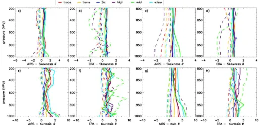
Fig. 6.The same as Fig. 5 except for the skewness and kurtosis.
is driven to a large extent by time variations and not spatial variations, unlike AIRS, which is primarily driven by spa-tial variations. In general,σθ is largest in the MBL and near
the tropopause for all cloud types in both AIRS and ERA-Interim. For high clouds, low values ofσare observed in the
MBL and near 250–300 hPa. On average, approximate Gaus-sian behavior ofθis observed for most of the ERA-Interim
profiles; this is suggested by low values of skewness and kur-tosis and random oscillations along the vertical profile. The exception is in the MBL, where a slightly higher variability in the higher moments is visible. Similar Gaussian behav-ior is observed for AIRS data in the case of Sc and trans Cu. Daily averages show a negative skewness for almost all cases, whereas the total skewness is close to zero. However, the kurtosis has a strong positive tendency in the satellite data in the MBL that is not seen in ERA-Interim.
AIRS cannot accurately resolve the fine vertical detail of the MBL (Maddy and Barnet, 2008). However, these results
demonstrate a systematic change in the distributional char-acteristics of θ between the MBL and free troposphere in
both clear and cloudy sky compared to ERA-Interim. Over-all, the observations by AIRS show structured patterns in the profile of the higher moments, whereas the variability is more random in the ERA-Interim data. This suggests that AIRS is resolving MBL structures that ERA-Interim is not capturing despite the known reduced sensitivity of AIRS in the lower troposphere and within the presence of high values of cloud fraction. Furthermore, a closer examination shows significant differences for the cloud types. First,σθ is
Fig. 7.The same as Fig. 5 except for the vertical profile of water vapor mixing ratio (g/kg).
Fig. 8.The same as Fig. 6 except for the vertical profile of water vapor mixing ratio (g/kg).
cloud-resolving model. They obtained large vertical varia-tions in the statistics of liquid water potential temperature (θl), total water mixing ratio (qt), and vertical velocity over
the depth of the cloud layer. A comparison of Zhu and Zuidema (2009) with AIRS suggests similarities ofθl and
θ in positive skewness of observed high clouds, similar to
the positive skewness seen in the simulations of the above authors. However, with respect to low clouds, AIRS cannot resolve the strong gradients at the top of the broken cloud layers shown in Zhu and Zuidema (2009), and this highlights the importance of obtaining higher-vertical-resolution ther-modynamic soundings than currently available from infrared and microwave satellite sounding.
3.4 Water vapor profiles
The statistical moments ofqare summarized in Figs. 7 and 8.
For AIRS, the mean profiles ofqshow drier conditions for Sc
and trans Cu than for trade Cu and clear sky and are less well mixed in the lowest levels. ERA-Interim and AIRS/MODIS
show very similar magnitudes and relative ordering of av-erage q sorted by MBL cloud type. AIRS shows a weaker
transition from the well-mixed boundary layer to the free tro-posphere in the mean profiles, similar to what we have seen already in the temperature profiles. Again, this is indication that the weakness of the current AIRS retrieval is the low sensitivity in the boundary layer caused by limits in the AIRS vertical resolution (Maddy and Barnet, 2008). The “average” profiles show a smoothed mean boundary layer profile ofq.
However, the higher moments are more sensitive to the devi-ations from the average, and we can quantify their behavior in the boundary layer with high confidence based on previous work (e.g., Kahn et al., 2011b; Yue et al., 2011). As expected, the standard deviation ofq(σq)in Fig. 7, panel e, is higher in
the MBL compared to the free troposphere for all AIRS cloud types. In the MBL (panel g), σq is relatively low for clear
sky and increasing from trade Cu to trans Cu to Sc. A subtle but notable feature in the AIRS data is a slight increase in
which coincides with the upper portion of the MBL near the base of the inversion. The ERA-Interim in panel h shows a similar but sharper gradient, which supports the assertion that AIRS is capable of capturing relative differences in the ver-tical structure ofσq.
There is also a notable difference between AIRS and ERA-Interim in the case of mid-level cloud in Fig. 7. ERA-ERA-Interim profiles have a much higher mean value and standard devia-tion ofq. There are two possible reasons for this. First, the
comparison of ERA-Interim with MODIS cloud data showed biases for mid-level clouds in ERA-Interim. ERA-Interim mid-level clouds appear more frequently compared to obser-vations (Fig. 3), and the higher values ofqare consistent with
their occurrence in low latitudes. Second, we restricted AIRS to “PGood” profiles with <=90 % cloud fraction. This limits the sample size and can result in an observational bias for the thickest clouds. This warrants a more detailed investigation of mid-level clouds in future work.
The skewness of AIRS and ERA-Interim (Fig. 8, panels a and b) is slightly positive for all cloud types and pressure levels on a daily average, but slightly negative for an overall skewness that accounts for time variations. The AIRS pro-files show an increase of this positive skewness within the free troposphere, similar to the kurtosis ofθ. This increase
is larger for Sc and trans Cu than for clear-sky and trade Cu cases, indicating that the lower latitudes, where trade Cu and clear sky occur, have stronger positively skewed profiles. ERA-Interim is almost constant throughout the troposphere, with slightly reduced values in the MBL. The kurtosis of
q shows high variations for AIRS observations. A large
in-crease is observed from Sc to trade Cu at 400 hPa. A qualita-tive comparison of AIRSqtoqtin Zhu and Zuidema (2009) is partly justified, as water vapor is the dominant component ofqt. An increase in skewness ofqtwith altitude is observed in Zhu and Zuidema (2009), consistent with observations of
q from AIRS. Furthermore, Iassamen et al. (2009) obtained
statistical moments of q from a ground-based microwave
profiler over land, dividing measurements into cloudy and clear cases. Similar variations in skewness and kurtosis of
q for cloud and clear-sky cases in the microwave
measure-ments and AIRS profiles are seen. Overall, the AIRS data, Zhu and Zuidema (2009), and Iassamen et al. (2009) collec-tively point towards a non-Gaussian cloud-type behavior of
qnot observed in ERA-Interim.
4 Conclusions
A novel pixel-scale application of cloud properties and ther-modynamic profiles obtained from the NASA Aqua MODer-ate resolution Imaging Spectroradiometer (MODIS) and At-mospheric Infrared Sounder (AIRS) is presented for a sub-tropical cloud regime transition in the northeastern Pacific Ocean. Simultaneous observations of cloud properties, po-tential temperature (θ )and water vapor (q)profiles are
quan-tified by cloud type for all available July days from 2003 to 2012. A collocation method that uses the prelaunch spatial response functions of AIRS is used to obtain robust cloud-type estimates within the AIRS field of view using MODIS cloud products. Cloud-type-dependent estimates of the sta-tistical properties of clouds and thermodynamic profiles are quantified. The focus is within the northeastern Pacific Ocean summertime along the GPCI cross section, a region well known for a persistent stratocumulus to trade cumulus tran-sition. This marine boundary layer cloud transition is con-sidered to be highly relevant to observational and model as-sessments of climate sensitivity. Individual AIRS FOVs are sorted into stratocumulus (Sc), transition cumulus (trans Cu), and trade cumulus (trade Cu), mid-level and high clouds, and clear sky. The mean, standard deviation, skewness and kurtosis of the cloud fields and thermodynamic profiles are obtained separately for each cloud type. AIRS and MODIS probability density functions (PDFs) are compared to simi-larly derived PDFs obtained from the ERA-Interim reanaly-sis.
The analysis of the observed PDFs and their higher mo-ments suggests the following:
– The average occurrence of MBL clouds relative to
clear sky is higher in ERA-Interim than in the obser-vations from MODIS.
– Cloud fraction distributions are significantly different
within the trade Cu, trans Cu and Sc cloud-type cate-gories between MODIS and ERA-Interim.
– The distribution of Tc for trade Cu in AIRS/MODIS has higher and more strongly skewed values than ERA-Interim
– A strong skewness in the LTS of low clouds is seen in
observations.
– LTS shows a PDF with strong skewness and bimodal
shape for clear-sky cases in the ERA-Interim data, which is not seen in observations.
– Clear sky and trade Cu both exhibit non-Gaussian
be-havior ofθ in observations, which is weaker in
ERA-Interim
– For q, reductions in the standard deviations are
ob-served in the MBL in ERA-Interim and observations.
– A positive skewness and kurtosis ofq in the free
tro-posphere is seen for observations but not for ERA-Interim.
– Both ERA-Interim and observations tend to have
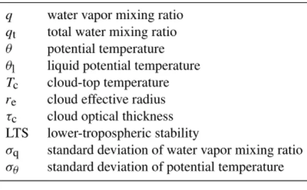
Table 3.Acronyms and symbols used in text.
q water vapor mixing ratio qt total water mixing ratio θ potential temperature θl liquid potential temperature Tc cloud-top temperature re cloud effective radius τc cloud optical thickness LTS lower-tropospheric stability
σq standard deviation of water vapor mixing ratio σθ standard deviation of potential temperature
– ERA-Interim shows reduced magnitudes in skewness
and kurtosis, indicating a more Gaussian behavior than observations.
Knowing the distributional characteristics of cloud and ther-modynamic properties for different types of clouds is nec-essary for implementing a subgrid-scale parameterization of cloud processes in climate models. The results obtained from the synergistic, pixel-scale MODIS and AIRS observa-tions offer important constraints on the spatial, temporal and cloud-type variability in these PDFs.
Future work will include an extension of this method to other MBL transitional regimes, as well as an expansion to other cloud regimes throughout the seasonal cycles over the NASA Aqua observing record.
Acknowledgements. Funding for this project was provided by NASA award NNX08AI09G. The authors would like to thank J. Teixeira and the AIRS project at the Jet Propulsion Labora-tory for encouragement and support. MODIS data were obtained through the Level-1 and Atmosphere Archive and Distribution Sys-tem (LAADS; http://ladsweb.nascom.nasa.gov/). AIRS data were obtained through the Goddard Earth Sciences Data and Informa-tion Services Center (http://daac.gsfc.nasa.gov). A porInforma-tion of this work was performed within the Joint Institute for Regional Earth System Science & Engineering (JIFRESSE) of the University of California, Los Angeles (UCLA), and at the Jet Propulsion Labora-tory, California Institute of Technology, under contract with NASA. We also would like to thank the reviewers for their valuable com-ments, which considerably helped in improving the quality of the manuscript.
The JPL author’s copyright for this publication is held by the California Institute of Technology. Government sponsorship is also acknowledged.
Edited by: A. Geer
References
Ackerman, S. A., Holz, R. E., Frey, R., Eloranta, E. W., Maddux, B. C., and McGill, M.: Cloud detection with MODIS. Part II: Validation, J. Atmos. Ocean. Tech., 25, 1073–1086, 2008. Ahlgrimm, M. and Köhler, M.: Evaluation of trade cumulus in
the ECMWF model with observations from CALIPSO, Mon. Weather Rev., 138, 3071–3083, 2010.
Albrecht, B. A., Bretherton, C. S., Johnson, D., Scubert, W. H., and Frisch, A. S.: The Atlantic Stratocumulus Transition Experiment–ASTEX, B. Am. Meteorol. Soc., 76, 889–904, 1995.
Aumann, H. H., Chahine, M. T., Gautier, C., Goldberg, M., Kalnay, E., McMillin, L., Revercomb, H., Rosenkranz, P. W., Smith, W. L., Staelin, D., Strow, L., and Susskind, J.: AIRS/AMSU/HSB on the aqua mission: Design, science objectives, data products, and processing systems, IEEE T. Geosci. Remote, 41, 253–264, 2003.
Barnes, W. L., Pagano, T. S., and Salomonson, V. V.: Prelaunch characteristics of the Moderate Resolution Imaging Spectrora-diometer (MODIS) on EOS-AM1, IEEE T. Geosci. Remote, 36, 1088–1100, 1998.
Bogenschutz, P. A., Gettelman, A., Morrison, H., Larson, V. E., Craig, C., and Schanen, D. P.: Higher-Order Turbulence Closure and Its Impact on Climate Simulations in the Community Atmo-sphere Model, J. Climate, 26, 9655–9676, doi:10.1175/JCLI-D-13-00075.1, 2013.
Bony, S. and Dufresne, J.-L.: Marine boundary layer clouds at the heart of tropical cloud feedback uncertainties in climate models, Geophys. Res. Lett., 32, L20806, doi:10.1029/2005GL023851, 2005.
Cess, R. D., Potter, G. L., Blanchet, J. P., Boer, G. J., Ghan, S. J., Kiehl, J. T., Treut, H. L., Li, Z.-X., Liang, X.-Z., Mitchell, J. F. B., Morcrette, J.-J., Randall, D. A., Riches, M., Roeckner, E., Schlesse, U., Slingo, A., Taylor, E. E., Washington, W. M., Wetherald, R. T., and Yagai, I.: Interpretation of cloud-climate feedback as produced by 14 atmospheric general circulation models, Science, 245, 513–516, 1989.
Cess, R. D., ,Zhang, M. H., Ingram, W. J., Potter, G. L., Alek-seev, V., Barker, H. W., Cohen-Solal, E., Colman, R. A., Da-zlich, D. A., Del Genio, A. D., Dix, M. R., Dymnikov, V., Esch, M., Fowler, L. D., Fraser, J. R., Galin, V., Gates, W. L., Hack, J. J., Kiehl, J. T., Le Treut, H., Lo, K. K.-W., McA-vaney, B. J., Meleshko, V. P., Morcrette, J.-J., Randall, D. A., Roeckner E., Royer, J.-F., Schlesinger, M. E., Sporyshev, P. V., Timbal, B., Volodin, E. M., Taylor, K. E., Wang, W., and Wetherald, R. T.: Cloud feedback in atmospheric general circu-lation models: An update, J. Geophys. Res., 101, 12791–12794, doi:10.1029/96JD00822, 1996.
Cuijpers, J. W. M., and Bechtold, P.: A simple parameterization of cloud water related variables for use in boundary layer models, J. Atmos. Sci., 52, 2486–2490, 1995.
ERA-Interim reanalysis: configuration and performance of the data assimilation system, Q. J. Roy Meteor. Soc., 137, 553–597, doi:10.1002/qj.828, 2011.
Frey, R. A., Ackerman, S. A., Liu, Y., Strabala, K. I., Zhang, H., Key, J. R., and Wang, X.: Cloud detection with MODIS. Part I: Improvements in the MODIS cloud mask for Collection 5, J. Atmos. Ocean. Tech., 25, 1057–1072, 2008.
Gerber, H.: Microphysics of marine stratocumulus clouds with two drizzle modes, J. Atmos. Sci., 53, 1649–1662, 1996.
Gierens, K., Kohlhepp, R., Dotzek, N., and Smit, H. G.: Instanta-neous fluctuations of temperature and moisture in the upper tro-posphere and tropopause region. Part 1: Probability densities and their variability, Meteorol. Z., 16, 221–231, 2007.
Guo, H., Golaz, J.-C., Donner, L. J., Larson, V. E., Schanen, D. P., and Griffin, B. M.: Multi-variate probability density func-tions with dynamics for cloud droplet activation in large-scale models: single column tests, Geosci. Model Dev., 3, 475–486, doi:10.5194/gmd-3-475-2010, 2010.
Hartmann, D., Ockert-Bell, M., and Michelsen, M.: The effect of cloud type on Earth’s energy balance: Global analysis, J. Cli-mate, 5, 1281–1304, 1992.
Iassamen, A., Sauvageot, H., Jeannin, N., and Ameur, S.: Distri-bution of tropospheric water vapor in clear and cloudy condi-tions from microwave radiometric profiling, J. Appl. Meteorol., 48, 600–615, 2009.
IFS documentation, Cy31r1, Part IV: physical processes, http://www.ecmwf.int/research/ifsdocs/CY31r1/PHYSICS/ IFSPart4.pdf (last access: 2 January 2014), 2007.
IPCC, Climate Change 2007: The Physical Science Basis. Con-tribution of Working Group I to the Fourth Assessment Report of the Intergovernmental Panel on Climate Change, edited by: Solomon, S., Qin, D., Manning, M., Chen, Z., Marquis, M., Av-eryt, K. B., Tignor, M., and Miller, H. L., Cambridge University Press, Cambridge, United Kingdom and New York, NY, USA, 2007.
Kahn, B. H, Nasiri, S. L., Schreier, M. M., and Baum, B. A.: Impacts of sub-pixel cloud heterogeneity on infrared ther-modynamic phase assessment, J. Geophys. Res., D20201, doi:10.1029/2011JD015774, 2011a.
Kahn, B. H., Teixeira, J., Fetzer, E. J., Gettelman, A., Hristova-Veleva, S. M., Huang, X., Kochanski, A. K., Köhler, M., Krueger, S. K., Wood, R., and Zhao, M.: Temperature and Water Vapor Variance Scaling in Global Models: Comparisons to Satellite and Aircraft Data, J. Atmos. Sci., 68, 2156–2168, doi:10.1175/2011JAS3737.1, 2011b.
Karlsson, J., Svensson, G., Cardoso, S., Teixeira, J., and Paradise, S.: Subtropical Cloud-Regime Transitions: Boundary Layer Depth and Cloud-Top Height Evolution in Models and Obser-vations, J. Appl. Meteorol., 49, 1845–1858, 2010.
Kawai, H. and Teixeira, J.: Probability density functions of liquid water path and cloud amount of marine boundary layer clouds: Geographical and seasonal variations and controlling meteoro-logical factors, J. Climate, 23, 2079–2092, 2010.
King, N. J., Bower, K. N., Crosier, J., and Crawford, I.: Evaluating MODIS cloud retrievals with in situ observa-tions from VOCALS-REx, Atmos. Chem. Phys., 13, 191–209, doi:10.5194/acp-13-191-2013, 2013.
Klein, S. A. and Hartmann, D. L.: The seasonal cycle of low strati-form clouds, J. Climate, 6, 1587–1606, 1993.
Lambrigtsen, B. H. and Lee, S.-Y.: Coalignment and synchroniza-tion of the AIRS instrument suite, IEEE T. Geosci. Remote, 41, 343–351, 2003.
Larson, V. E., Wood, R., Field, P. R., Golaz, J.-C., Vonder Haar, T. H., and Cotton, W. R.: Small-Scale and mesoscale variability of scalars in cloudy boundary layers: One-dimensional probability density functions, J. Atmos. Sci., 58, 1978–1994, 2001. Lewis, E. R., Wiscombe, W. J., Albrecht, B. A., Bland, G. L.,
Flagg, C. N., Klein, S. A., Kollias, P., Mace, G., Reynolds, R. M., Schwartz, S. E, Siebesma, A. P., Teixeira, J., Wood, R., and Zhang, M.: MAGIC: Marine ARM GPCI Investiga-tion of Clouds, Environmental Sciences, DOE/SC-ARM-12-020, http://www.osti.gov/scitech/servlets/purl/1052589 (last access: 1 April 2014), 2012.
Li, J., Menzel, W. P., Sun, F., Schmit, T. J., and Gurka, J.: AIRS subpixel cloud characterization using MODIS cloud products, J. Appl. Meteorol., 43, 1083–1094, 2004a.
Li, J., Menzel, W. P., Zhang, W., Sun, F., Schmit, T. J., Gurka, J. J., and Weisz, E.: Synergistic use of MODIS and AIRS in a variational retrieval of cloud parameters, J. Appl. Meteorol., 43, 1619–1634, 2004b.
Maddy, E. S. and Barnet, C. D.: Vertical resolution estimates in ver-sion 5 of AIRS operational retrievals. IEEE T. Geosci. Remote, 46, 2375–2384, 2008.
Maddy, E. S., King, T. S., Sun, H., Wolf, W. W., Barnet, Heidinger, A., Cheng, Z., Goldberg, M. D., Gambacorta, A., Zhang, C., and Zhang, K.: Using Metop-A AVHRR clear-sky measurements to cloud-clear Metop-A ISAI column radiances, J. Atmos. Ocean. Tech., 28, 1104–1116, doi:10.1175/JTECH-D-10-05045.1, 2011. Marchand, R., Ackerman, T., Smyth, M., and Rossow, W. B.: A review of cloud top height and optical depth histograms from MISR, ISCCP, and MODIS, J. Geophys. Res., 115, D16206, doi:10.1029/2009JD013422, 2010.
Martins, J. P. A., Teixeira, J., Soares, P. M. M., Miranda, P. M. A., Kahn, B. H., Dang, V. T., Irion, F. W., Fetzer, E. J., and Fishbein, E.: Infrared sounding of the trade-wind boundary layer: AIRS and the RICO experiment, Geophys. Res. Lett., 37, L24806, doi:10.1029/2010GL045902, 2011.
Masunaga, H., Nakajima, T. Y., Nakajima, T., Kachi, M., and Suzuki, K.: Physical properties of maritime low clouds as re-trieved by combined use of Tropical Rainfall Measuring Mis-sion (TRMM) Microwave Imager and Visible/Infrared Scanner, 2. Climatology of warm clouds and rain, J. Geophys. Res., 107, 4367, doi:10.1029/2001JD001269, 2002.
Medeiros, B., Stevens, B., Held, I. M., Zhao, M., Williamson, D. L., Olson, J. G., and Bretherton, C. S.: Aquaplanets, climate sensi-tivity, and low clouds, J. Climate, 21, 4974–4991, 2008. Menzel, W. P., Baum, B. A., Strabala, K. I., and Frey, R. A.: Cloud
top properties and cloud phase, MODIS Algorithm Theoretical Basis Document, 2006.
Nasiri, S. L., Dang, H. V. T., Kahn, B. H., Fetzer, E. J., Manning, E. M., Schreier, M. M., and Frey, R. A.: Comparing MODIS and AIRS infrared-based cloud retrievals, J. Appl. Meteorol. Clim., 50, 1057–1072, 2011.
Ou, S.-C., Kahn, B. H., Liou, K. N., Takano, Y., Schreier, M. M., and Yue, Q.: Retrieval of cirrus cloud properties from the At-mospheric Infrared Sounder: The k-coefficient approach com-bined with SARTA plus delta-four stream approximation, IEEE T. Geosci. Remote, 1010–1024, 2013.
Overoye, K., Aumann, H. H., Weiler, M. H., Gigioli, G. W., Shaw, W., Frost, E., and McKay, T.: Test and Calibration of the AIRS instrument, SPIE Proceedings, 3759, 254–265, 1999.
Pincus, R., and Klein, S. A.: Unresolved spatial variability and mi-crophysical process rates in large-scale models, J. Geophys. Res., 105, 27059–27065, 2000.
Platnick, S., King, M. D., Ackerman, S. A., Menzel, W. P., Baum, B. A., Riédi, J. C., and Frey, R. A.: The MODIS cloud products: Algorithms and examples from Terra, IEEE T. Geosci. Remote, 41, 459–473, 2003.
Pressel, K. G. and Collins, W. D.: First order structure function anal-ysis of statistical scale invariance in the observed AIRS water vapor field, J. Climate, 25, 5538–5555, 2012.
Price, J. D., and Wood, R.: Comparison of probability density func-tions for total specific humidity and saturation deficit humidity, and consequences for cloud parameterization, Q. J. Roy. Meteor. Soc., 128, 2059–2072, 2002.
Quaas, J.: Evaluating the “critical relative humidity” as a measure of subgrid-scale variability of humidity in general circulation model cloud cover parameterizations using satellite data, J. Geophys. Res, 117, D09208, doi:10.1029/2012JD017495, 2012.
Randall, D. A.: Beyond deadlock, Geophys. Res. Lett., 40, 5970– 5976, doi:10.1002/2013GL057998, 2013.
Rossow, W. B. and Schiffer, R. A.: Advances in Understanding Clouds from ISCCP, B. Am. Meteorol. Soc., 72, 2–20, 1999, Schreier, M. M., Kahn, B. H., Eldering, A., Elliott, D. A.,
Fish-bein, E., Irion, F. W., and Pagano, T. S.: Radiance comparisons of MODIS and AIRS using spatial response information, J. At-mos. Ocean. Tech., 27, 1331–1342, 2010.
Slingo, J. M.: A cloud parametrization scheme derived from GATE data for use with a numerical model, Q. J. Roy. Meteor. Soc., 106, 747–770, doi:10.1002/qj.49710645008, 1980.
Sommeria, G. and Deardorff, J. W.: Subgrid-scale condensation in models of nonprecipitating clouds, J. Atmos. Sci., 34, 344–355, 1977.
Stephens, G. L.: Cloud feedbacks in the climate system: A critical review, J. Climate, 18, 237–273, 2005.
Stevens, B.: Atmospheric Moist Convection, Annu. Earth Planet. Sci., 32, 605–643, 2005.
Stevens, B., Lenschow, D. H., Vali, G., Gerber, H., Bandy, A., Blomquist, B., Brenguier, J.-L., Bretherton, C. S., Burnet, F., Campos, T., Chai, S., Faloona, I., Friesen, D., Haimov, S., Laursen, K., Lilly, D. K., Loehrer, S. M., Malinowski, S. P., Morley, B., Petters, M. D., Rogers, D. C., Russell, L., Savic-Jovcic, V., Snider, J. R., Straub, D., Szumowski, M. J., Tak-agi H., Thornton, D. C., Tschudi, M., Twohy, C., Wetzel M., and van Zanten, M. C.: Dynamics and Chemistry of Marine Stratocumulus–DYCOMS-II, B. Amer. Meteorol. Soc., 84, 579– 593, doi:10.1175/BAMS-84-5-579, 2003.
Su, H., Jiang, J. H., Vane, D. G., and Stephens, G. L.: Ob-served vertical structure of tropical oceanic clouds sorted in large-scale regimes, Geophys. Res. Lett., 35, L24704, doi:10.1029/2008GL035888, 2008.
Sukhatme, J. and Young, W. R.:The advection-condensation model and water vapour PDFs, Q. J. Roy. Meteorol. Soc., 137, 1561– 1572, doi:10.1002/qj.869, 2010.
Susskind, J., Barnet, C. D., and Blaisdell, J. M.: Retrieval of atmo-spheric and surface parameters from AIRS/AMSU/HSB data in the presence of clouds, IEEE T. Geosci. Remote, 41, 390–409, 2003.
Susskind, J., Barnet, C., Blaisdell, J., Iredell, L., Keita, F., Kouvaris, L., Molnar, G., and Chahine, M.: Accuracy of geophysical pa-rameters derived from Atmospheric Infrared Sounder/Advanced Microwave Sounding Unit as a function of fractional cloud cover, J. Geophys. Res., 111, D09S17, doi:10.1029/2005JD006272, 2006.
Teixeira, J., Cardoso, S., Bonazzola, M., Cole, J., DelGenio, A., De-Mott, C., Franklin, C., Hannay, C., Jakob, C., Jiao, Y., Karlsson, J., Kitagawa, H., Koehler, M., Kuwano-Yoshida, A., Ledrian, C., Lock, A., Miller, M. J., Marquet, P., Martins, J., Me-choso, C. R., Meijgaard, E. V., Meinke, I., Miranda, P. M. A., Mironov, D., Neggers, R., Pan, H. L., Randall, D. A., Rasch, P. J., Rockel, B., Rossow, W. B., Ritter, B., Siebesma, A. P., Soares, P., Turk, F. J., Vaillancourt, P., Von Engeln, A., and Zhao, M.: Tropical and subtropical cloud transitions in weather and climate prediction models: the GCSS/WGNE Pacific Cross-section Inter-comparison (GPCI), J. Climate, 24, 5223–5256, doi:10.1175/2011JCLI3672.1, 2011.
Tobin, D. C., Revercomb, H. E., Moeller, C. C., and Pagano, T. S.: Use of AIRS high spectral resolution spectra to assess the calibration of MODIS on EOS Aqua, J. Geophys. Res., 111, D09S05, doi:10.1029/2005JD006095, 2006.
Tompkins, A. M.: Impact of temperature and humidity variability on cloud cover assessed using aircraft data. Q. J. Roy. Meteorol. Soc., 129, 2151–2170, doi:10.1256/qj.02.190, 2003.
Uppala, S. M., KÅllberg, P. W., Simmons, A. J., Andrae, U., Bech-told, V. D. C., Fiorino, M., Gibson, J. K., Haseler, J., Hernandez, A., Kelly, G. A., Li, X., Onogi, K., Saarinen, S., Sokka, N., Allan, R. P., Andersson, E., Arpe, K., Balmaseda, M. A., Beljaars, A. C. M., Berg, L. V. D., Bidlot, J., Bormann, N., Caires, S., Chevallier, F., Dethof, A., Dragosavac, M., Fisher, M., Fuentes, M., Hage-mann, S., Hólm, E., Hoskins, B. J., Isaksen, L., Janssen, P. A. E. M., Jenne, R., Mcnally, A. P., Mahfouf, J.-F., Morcrette, J.-J., Rayner, N. A., Saunders, R. W., Simon, P.,Sterl, A., Trenberth, K. E., Untch, A., Vasiljevic, D., Viterbo, P., and Woollen, J.: The ERA-40 re-analysis, Q. J. Roy. Meteorol. Soc., 131, 2961–3012, doi:10.1256/qj.04.176, 2005.
Vial, J., Dufresne, J.-L., and Bony, S.: On the interpretation of inter-model spread in CMIP5 climate sensitivity estimates, Clim. Dy-nam., 41, 3339–3362, 2013.
Weber, T., Quaas, J., and Räisänen, R.: Evaluation of the statistical cloud scheme in the ECHAM5 model using satellite data, Q. J. Roy. Meteorol. Soc., 137, 2079–2091, 2011.
Williams, K. D. and Webb, M. J.: A quantitative performance as-sessment of cloud regimes in climate models. Clim. Dynam., 33, 141–157, doi:10.1007/s00382-008-0443-1, 2009.
Wood, R., and Bretherton, C. S.: On the relationship between strat-iform low cloud cover and lower-tropospheric stability, J. Cli-mate, 19, 6425–6432, 2006.
cli-mate change in three AGCMs sorted into regimes using mid-tropospheric vertical velocity, Climate Dynam., 27, 261–279, doi:10.1007/s00382-006-0138-4, 2006.
Yue, Q., Kahn, B. H., Fetzer, E. J., and Teixeira, J.: Relationship between oceanic boundary layer clouds and lower tropospheric stability observed by AIRS, CloudSat, and CALIOP, J. Geophys. Res., 116, D18212, doi:10.1029/2011JD016136, 2011.
Yue, Q., Fetzer, E., Kahn, B., Wong, S., Manipon, G., Guillaume, A., and Wilson, B.: Cloud-state-dependent Sampling in AIRS Observations based on CloudSat Cloud Classification, J. Cli-mate, 26, 8357–8377, doi10.1175/JCLI-D-13-00065.1, 2013.
Zhang, C., Mapes, B. E., and Soden, B. J.: Bimodality in tropical water vapor, Q. J. Roy. Meteorol. Soc., 129, 2847–2866, 2006. Zhao, G. and Di Girolamo, L.: Cloud fraction errors for trade wind
cumuli from EOS-Terra instruments, Geophys. Res. Lett., 33, L20802, doi:10.1029/2006GL027088, 2006.