Ongoing Processes in a Fitness Network
Model under Restricted Resources
Takayuki Niizato1*, Yukio-Pegio Gunji2
1Faculty of Engineering, Information and Systems, Tsukuba University, Tsukuba, Ibaraki, Japan,2School of Fundamental Science and Engineering, Waseda University, Tokyo, Japan
Abstract
In real networks, the resources that make up the nodes and edges are finite. This constraint poses a serious problem for network modeling, namely, the compatibility between robust-ness and efficiency. However, these concepts are generally in conflict with each other. In this study, we propose a new fitness-driven network model for finite resources. In our model, each individual has its own fitness, which it tries to increase. The main assumption in fitness-driven networks is that incomplete estimation of fitness results in a dynamical growing network. By taking into account these internal dynamics, nodes and edges emerge as a result of exchanges between finite resources. We show that our network model exhibits exponential distributions in the in- and out-degree distributions and a power law distribution of edge weights. Furthermore, our network model resolves the trade-off relationship be-tween robustness and efficiency. Our result suggests that growing and anti-growing net-works are the result of resolving the trade-off problem itself.
Introduction
Many evolving network models are based on the well-known property of preferential attach-ment [1,2,3]. We regard the main rule for preferential attachment in evolving network models as being constructed from at least the following two working concepts. (i) A new node is added to the network at every step, and (ii) a fixed number of edges are connected to existing nodes that have more connections than others (i.e. the probability of connecting a new edge between the new node and an existing node is proportional to the number of edges already connected to the existing node). Rule (ii) in particular suggests that new edges from new nodes preferentially attach to old nodes when these existing nodes have many links (the so-called rich-get-richer ef-fect). For this reason, the set of rules (i) and (ii) is called preferential attachment. It has already been found that the heterogeneous connectivity of the network emerges from this preferential attachment. The scale-free network structure, in particular, is considered a ubiquitous property of the structure of many real networks. Preferential attachment is a good tool for determining the power laws in the structure of networks [2,3].
The concept of preferential attachment has been criticized by many researchers [4,5,6,7,8,
9]. Mandelbrot, for example, criticized the mechanical aspect of preferential attachment (more OPEN ACCESS
Citation:Niizato T, Gunji Y-P (2015) Ongoing Processes in a Fitness Network Model under Restricted Resources. PLoS ONE 10(5): e0127284. doi:10.1371/journal.pone.0127284
Academic Editor:Celine Rozenblat, UNIVERSITY
OF LAUSANNE, SWITZERLAND
Received:October 17, 2014
Accepted:April 13, 2015
Published:May 18, 2015
Copyright:© 2015 Niizato, Gunji. This is an open access article distributed under the terms of the
Creative Commons Attribution License, which permits unrestricted use, distribution, and reproduction in any medium, provided the original author and source are credited.
Data Availability Statement:All relevant data are within the paper and its Supporting Information files.
Funding:The authors have no support or funding to report.
Competing Interests:The authors have declared
specifically, the preferential attachment-like models proposed in the past) and pointed out the lack of any underlying mechanism [4]. We thus analyze the method behind the concept of pref-erential attachment. We point out that there are two hidden assumptions behind the two rules that we listed. One is that a newly added node can make a quick overall observation of informa-tion about the whole network because otherwise it would need to know the degree distribuinforma-tion of a given network in advance in order to distinguish the more popular nodes from the others. The other is the assumption that the number of nodes and edges in a given network always in-creases because the preferential attachment algorithm always adds a new node and a fixed number of edges to the network.
The first hidden assumption has been pointed out by many researchers [5,6,7,8,9]. Re-searchers who have tried to resolve this problem have introduced internal dynamics to nodes and added edges by many different processes. Although there are many approaches to this problem, we consider that a common approach is to limit the selection of nodes when using preferential attachment. In other words, the nodes selected from the population are restricted by taking into account the activation of the node, aging, and locality selection, which is called a
“local world”[5,6,7]. This kind of restriction on the selection of nodes prevents us from pre-suming global information about the degree distribution of nodes. All a new node needs to do is to seek more popular nodes from this limited set of nodes. Of course, these approaches are an extension of preferential attachment.
Unlike the first hidden assumption, the second one is seldom discussed. Real networks such as the World Wide Web (WWW) [10,11] and social networks [12,13,14], are indeed expected to grow virtually without limit. However, if we look at other real networks, we discover that cases of networks that grow forever are rare. For example, ecological networks have at most two hundred nodes (species) and a thousand edges (such as the flow of carbon or energy) [15,
16,17]. This fact also applies to airport transportation networks [18] and protein reaction net-works [19]. In these cases, we cannot expect an ever-growing network like the WWW. With re-spect to the WWW, the important point of the listed network is the temporal dynamics of the networks, that is, the increases and decreases in the number of nodes and edges, since the nodes and edges in ecological networks and other networks change with time due to the effect of external perturbations such as extinction events.
However, we need to point out here the radical assumption of the evolving network model. The radical assumption in preferential attachment is that most models admit an asynchronous update rule in their algorithms [1,2]. In other words, there is no change in the network dynam-ics without the addition of new nodes and selected existing nodes. By using an asynchronous updating rule, we are able to obtain perfect information about network structures, such as the degree distribution, and to construct algorithms for preferential attachment. We feel that this problem is critical because protein reaction networks and networks of energy flows between species involve events on many timescales, with these multi-scale processes occurring at the same time. Furthermore, the study of network theory is motivated by attempting to understand these many possible processes as a whole system.
We thus propose a new model for evolving networks. Our network model is constructed by individuals who have their own fitness which is determined by their environment. Each indi-vidual belongs to one state (this corresponds to being a node in the network). Each indiindi-vidual tries to raise its own fitness and change its state. These state transitions of individuals create a weighted state transition network which dynamically changes with time. Our network model exhibits an asymmetrical relationship between the in-degree and out-degree distributions. Fur-thermore, the dynamical aspect of our evolving network model leads us to consider a develop-mental process in the network (growing and decaying) with time.
The paper consists of the following sections. In section 2, we explain the algorithm used in the model and how the state transition network is constructed. Our model uses lattice theory, which is often employed in computer science. The basic notion of lattice theory is detailed in
S1 Text. In Section 3, we analyze the evolving network in our model such as in terms of cluster-ing coefficient, degree distribution, and the trade-off relation between the mean degree (MD; diversity of states) and variance of edge weights (the overall gain in fitness). Finally, we discuss a developmental cycle in the network of our model.
Methods
Construction of the Model
Before we construct the network, we describe the underlying dynamics of the transition net-work. We assign each individual ann-bit binary string, and represent each individual by s1s2s3. . .snandsi2{0, 1} for alli2{1, 2,. . .,n}. For brevity, we denotes1s2s3. . .snbyhsin. Each bit string represents a state to which each individual belongs. If two individuals have the same bit string, then these two individuals belong to the same state. In our model, each individual tries to adapt to an environment, which is represented by the target bit strings (we denotehtin, i.e. t1t2t3. . .tn), through its interactions. We assign the values of the target bit strings at random. The adaptive process of each state in our model is the process by which each individual at-tempts to change its state into the target bit stringhtin. Because of the existence of the target bit strings, we can define the fitness of each individual. The fitness measures the degree of adapta-tion of an individual to its environment. In other words, if the bit string of an individual matches the target bit string well, then it has high fitness for the environment. The fitness of each individual is therefore defined by the Hamming distance from the target. Mathematically, we compute the fitness of each individual as follows.
Definition 1. (Fitness Bit String) Lethsinandhtinben-bit strings wherehsinis the state to which an individual belongs andhtinis the target. Letkbe a hidden digit in the target bit string.
For 1jn,
bj¼
0ðif s
j ¼tj and j6¼kÞ
1 ðif s
j6¼tj and j6¼kÞ
0or1randomlyðotherwiseÞ
8 > < > :
We callhbinthefitness bit strings for the target.
We therefore have three distinct types of bit strings. The first type is bit strings representing the state of an individual (denotedhsin). The second type is bit strings representing the fitnesses of individuals (denotedhbin). The last type is bit strings representing a target (denotedhtin). The main difference among them is that the first two (statehsinand fitnesshbin) types of bit string change over time, whereas the target bit stringhtinis fixed throughout each trial.
instance, 100111). The order relation between two binary bit strings is defined byhain hbinifaibifor alli2{1, 2,. . ..,n}. An important of property of partial ordered sets is the pos-sible existence of pairs of elements that are incomparable (for instance, 101 and 010 are incom-parable because 101 is larger than 010 at the first digit but smaller than 010 at the second digit). The concept of hidden digits in Definition 1 represents imperfect knowledge about the envi-ronment. In other words, each individual never has perfect knowledge about its envienvi-ronment. Each individual can only observen-1 bits of ann-bit target string. The fitness value of the hid-den position is determined randomly (zero or one). The position of the hidhid-den digit changes randomly from the first digit tonth digit at every step. If the position of a hidden digit isk(i.e. thek-th digit in a target bit stringhtin) at timet, each individual can observe the target bit string t1t2. . .tk-1tk+1. . .tn. Each individual tries to adapt to the uncertain environment by changing its state. Since an individual tries to raise its own fitness, it leaves its states the same (sjt+1=sjt) if it has high fitness digits (bj= 1) and changes its states randomly (sjt+1= 0 orsjt+1= 1) if it has low fitness (bj= 0). The idea of using a fitness measure for each state in a network is not new [22,23,24,25].
Unlike previous fitness models, we assume no particular distribution function for fitness [22,23]. In these models, the fitness information for each node is completely given. In contrast, the positioning of fitness in our model is utterly different because each individual lacks com-plete information (i.e. hidden digit) about its own fitness. Each individual tries to estimate its own fitness from incomplete information [26]. Taking this into account, the main difference in the attitude toward fitness is whether the fitness is given passively (fitness is given to a node as perfect information) or actively (fitness is given to a node as imperfect information). We con-struct this fitness during the development of the network as described in a later section.
Next we discuss the fitness dynamics in terms of the interactions between states. We repre-sent the fitness dynamics by using a quotient lattice from lattice theory (details of the definition of the quotient lattice are described inS1 Text). By using a quotient lattice, the fitness of each individual is never only determined by a local estimate, but also by a global estimate. The con-cept of quotient lattice is not difficult. The quotient lattice is a way of grouping a complete lat-tice (S1 Text). In lattice theory, a lattice is defined as a partially ordered set which is closed under the operations of join and meet. Roughly speaking, this implies the existence of bottom and top elements in a partially ordered set. In terms of fitness, the top element means high fit-ness overall. If an individual attains the highest fitfit-ness, there is thus no need to change state. Al-though it is generally difficult for individuals to achieve the highest fitness, we found that our algorithm made it possible for individuals to easily obtain the highest fitness despite the exis-tence of individuals whose fitness isnotthe highest.
According to Theorem 1.11 (seeS1 Text), we can obtain a unique quotient lattice if we take one element from a lattice. This grouping result, that is, the quotient lattice, corresponds to the global fitness. Generally, fitness cannot be determined only by local estimation (comparing with only a target bit string), but requires taking the global context into consideration. In this respect, a lattice for fitness corresponds to a global structure of fitness, and a quotient lattice for fitness corresponds to a global estimation. Mathematically, we can represent the fitness of each individual in a global context as follows.
Definition 2. (Fitness Being Induced by a Quotient Lattice) LetLbe a lattice ofn-bit strings,Jbe an ideal andθ(J) be a congruence on latticeL. For 1iN,
hbii;t
n _fhxi k;t n 2L
tjhxik;t n 2 ½hci
j;t
nyðJÞsuch thathbi
i;t n 2 ½hci
j;t nyðJÞg
congruenceθ(J). Therefore, a binary bit string offitness blocks is replaced by thelargest ele-mentin the congruence to which it belongs.
Details of the definition of an ideal, congruence, and join are listed inS1 Text. We only point out here that each individual takes the largest element to which it belongs in a given quo-tient lattice. Taking the largest element (i.e. fitness) against the original fitness estimated by local incomplete information means that each individual overestimates its own fitness when we take into account the global context for fitness estimation. However, this overestimation never indicates that the fitness actually increased. The overestimation of fitness is a kind of errorinduced by considering the global context. Each individual uses this overestimated fitness to change its state. The main effect of fitness overestimation is to suppress the degree of change in an individual state. For example, assuming we have a 3-bit string 100 (the state of an individ-ual) and its fitness 001 (the fitness of an individindivid-ual), this individual randomly flips the corre-sponding digits, that is, the 10 of 100. There are thus four possible changes (from 100 to 100, 110, 010, or 000). If overestimation of the fitness of this individual occurs due to the global con-text, such as if the fitness becomes 011, then there are only two patterns of change (from 110 to 010 or 110).
We briefly summarize the algorithm from our model.
1. GenerateN= 2nn-bit stringshsi
n1,0,hsin2,0,. . .hsinN,0and a targetn-bit stringhtinrandomly. The target is fixed through one trial. Note that these bit strings may be bitwise-identical (i.e. hsini,0=hsinj,0but be distinct as individualsiandj).
2. Randomly select a hidden digit of the target from the set {1, 2,. . .,n}. A fitness is formed from a set ofn-bit stringsBt= {hbin1,t,hbin2,t,. . .,hbinN,t} using Definition 1.1.
3. Create a latticeLtfrom thisBt.
4. Select one elementhb0i
ntin the latticeLtand create an ideal#hb0int.
5. Construct a quotient lattice from the idealJ=#hxint.
6. Substitute new binary bit strings of fitness blocks using Definition 2.
7. Change eachn-bit string using fitness blocks. For 1jn,
si;tþ1
j ¼
si;t j ðifb
i;t j ¼1Þ
0or1randomlyðotherwiseÞ
(
Construct a new set of binary bit strings for speciesBt+1= {hsin1,t+1,hsin2,t+1,. . .,hsinN,t+1}. The sequence of steps (2)-(7) forms one time step of a trial. Repeating steps (2)-(7), we can observe the evolution of the state and the lattice. Details of the algorithm are listed inS1 Text. The state in our model thus forms a lattice from local incomplete information, with fitness re-estimated from the global estimate, which is derived from a quotient lattice. The important point is that an individual never asynchronously updates its state. All individuals estimate their fitness and change state at the same time.
Creating a Transition Network
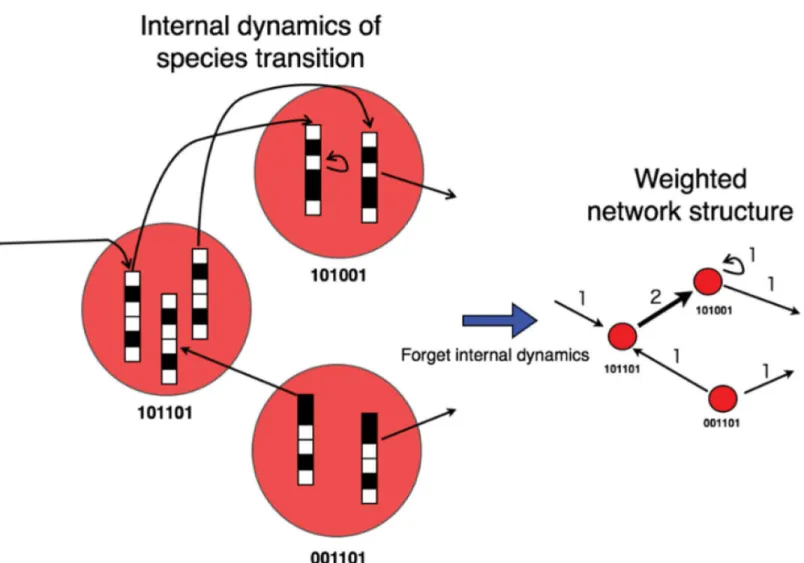
construction of a state transition in a network. The edge is formed by actual transitions in a cer-tain interval (one step inFig 1). The number above each edge represents its weight. From this example, it can be found that the sum of the weights of all edges is always fixed because all indi-viduals change state every step. Therefore, if there are 32 indiindi-viduals, then there are 32 state transitions which correspond to the edges. This can be expressed mathematically as follows:
k<s>n!<s0>nkw
¼X
t2
t¼t1
j<si>tn!<si>tnþ1 occur at timetwhen <s>n¼<si>tn and <s0>n¼<si>tnþ1 j
where ||-||wmeans the weight of the edge which corresponds to the state transitionhsint!hsint +1and
t2-t1is afixed interval of time. If we take enough time intervals (200 steps in this paper), we can obtain a fully connected directed weighted network (in this case, the total weight of edges is 200N.Nis the total number of individuals).
Fig 1. Example of the state transitions of all individuals.Constructing a network from the state transitions of all individuals. In this example, the network is constructed in one step from the state transition shown on the left. Bit strings (colored black for 0 and white for 1) represent individuals and red circles represent states (i.e. nodes). Individuals who have the same state are shown in the same circle. Arrows indicate transitions of individual induced fitness. The figure on the right represents the state transition network. Numbers above edges indicate the weights of the edges. The network contains a self-loop. Note the number of individuals (i.e. 2n
) never change with time but only the number of states.
We note that the transition network never satisfies the transitive property (if A implies B and B implies C, then A implies C) of edges. The possibility of transition exists in the network where a triangle relationship exists. Because of the fixed sum of weights, the weighted network suggests a trade-off relationship between the gain of all individuals (which corresponds to high overall fitness) and the resource distribution (which corresponds to a high diversity of species). This problem is discussed in a later section.
Results
Cluster Coefficient and Local Cluster Coefficient
Before we analyze the properties of the network of our model, we construct a control model with behavior that can be controlled by tuning one parameter. Since the details of the algorithm of the control model are listed inS1 Text, at this point we note that the concept of the model is to have a way of measuring fitness which can be controlled by one parameter. This parameter controls the error rate. The error rate is defined in terms of the probabilityμthat a digit that is the same in an individual as in the target bit string changes value. For example, we again con-sider three-bit strings (with 100 for the state and 011 for the fitness). Each of the "1" digits in this fitness (i.e. the last of two 1s) changes to 0 with probability 1-μ. The error rate therefore in-creases asμincreases. Therefore, by tuning this parameterμ, we can control the behavior of the species to mimic our evolving lattice (EL) model. Furthermore, because of this algorithm, high fitness states tend to become linked with each other without using any global information (fit-ness is determined by using only a target bit string). This model corresponds to a PA-like model under a finite resource environment. Compared with this control, the effect of using a lattice structure in our model becomes clearer.
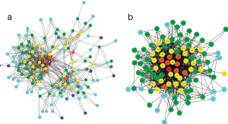
Fig 2A and 2Bshow two networks from our EL model and one example of the control model (parameters are fixed atμ= 0.005). All data in this paper are averages from over 100 times trials for the EL model and the control. As is shown in a later section, the state of the con-trol model when the parameterμis 0.005 is near the EL model compared with other parameter values (seeS1andS2Figs). We point out here the difference can be observed as a network structure (i.e. cluster coefficient). First, the global cluster coefficient of the control is four times larger than that of our model (C= 0.133 ± 0.020 for the EL model andC= 0.474 ± 0.028 for the control). In the same way, the mean degree of the control is two times larger than that of our model (MD = 5.00 ± 0.50 for the EL model and MD = 9.25 ± 0.32 for the control). This fact suggests the possibility that the state transition is restricted in the EL model. Compared with the EL model, the state transitions of the control are only controlled by one parameter. There-fore, the transition of species is determined statistically and never depends on the global con-text of the whole process. However, state transitions in the EL network are determined not only in a statistical way, but also from the lattice structure. Owing to the lattice structure (or re-placing each fitness with the top element of the quotient lattice), the possibility of state transi-tions never becomes free like in the control model.
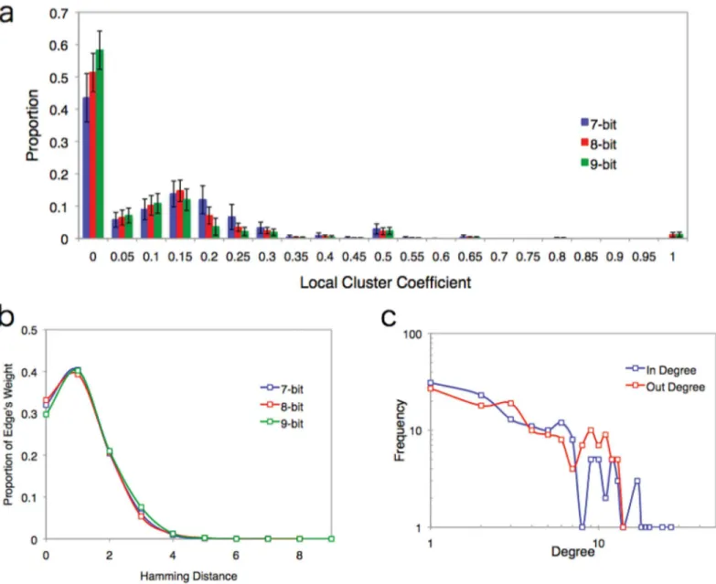
distance from the target are concentrated in small Hamming distance nodes (about 70% of a total weight of edge within 3 bits).
Weight and Degree Distribution of the Evolving Lattice Model
Next we examined two frequency distributions for in-degree and out-degree because it is given that the network is directed. However, the shapes of the degree distributions are constructive (Fig 3C). It seems that the slope of in-degree (λ
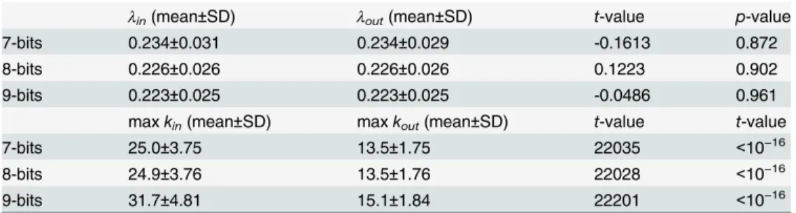
in) is steeper than that of out-degree (λout), but the statistical values are the same, withλin= 0.226 ± 0.026 andλout= 0.226 ± 0.026 (the detail of statistical test are listed onTable 1). However, the distribution of the tail position (i.e. the highest degree in the EL network in a certain interval) of in-degree (maxkin) is much larger than that of out-degree (maxkout) (SeeTable 1). In other words, there is an asymmetrical rela-tionship between the in-degree and out-degree distributions. This difference comes from the fitness algorithm of the EL network. Since each individual changes its state to increase its fit-ness, there are some nodes (state) that attract more edges than others. This popularity of nodes creates a ranking among all the nodes in the network. In contrast, the case of out-degree distri-bution is not related to the fitness algorithm of our model like the case of in-degree distribu-tion. The out-flow and in-flow in the network obey the different underlying mechanism when the degree distribution is constructed. We note that low cluster coefficient and exponential decay of degree distributions are observed in the WWW [10,11].
Fig 2. Examples of a network structure for the EL model (a) and the control (b). (a)The network of the EL network. Node colors represent the Hamming distance from the target bit string. Number in circles indicate the state. There are six colors, which are red (0), orange (1), yellow (2), green (3), light blue (4), and blue (5). The color of the target is red because the Hamming distance is zero. The global cluster coefficient and mean degree of the control network are much larger than those of our model. The number of nodes is always smaller than max possible nodes (i.e. 2n
) because many low fitness states may not be selected. In this figure, the total number of node is 142 (EL model) and 168 (Control).(b)The control network (μ= 0.005). Colors are the same as Fig. 2A.
Next we investigate the frequency distribution of weights. Most real networks are weighted networks [18,21,27]. The examples of ecosystems and social communities, where weak links play an important role in the stability of the network, are often cited [21]. However, despite the importance of weighted networks, most studies focus on unweighted networks. Many research-ers construct weighted networks by using a preferential attachment method, the same as un-weighted networks [29,30,31,32,33]. As we discussed before, our model is not preferential attachment because the update rule is synchronous. Despite the synchronous update rule, it is not a given that time progress will occur at each individual because some individuals may change at timetand some individuals may remain in the same state (digits) at timet. In this network, the weight of an edge is measured by counting state transition events in a certain time
Fig 3. Details of data for the EL network. (a)Distribution of the local cluster coefficient in the EL network. The horizontal axis corresponds to the local cluster coefficient (binned at 0.005) and the vertical axis corresponds to the proportion.(b)The proportion of edge weights for each Hamming distance. A large proportion of edge weights are concentrated within 3 bits. This tendency is the same in all cases.(c)The in-degree and out-degree degree distributions for the EL network. Both graphs show an exponential decay and the same scaling parameterλin= 0.226±0.026 andλout= 0.226±0.026. We use a maximum likelihood estimation method with a discrete distribution [27,28].
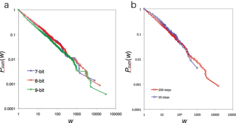
interval (200 steps in this study). We examined the frequency distribution of edge weights in
Fig 4A. The graph exhibits a power law distribution with a scaling exponent of 1.5. This power law behavior never depends on the number of bits (seeTable 2). Additionally, the power law distribution of our model never depends on the length of the time interval (Fig 4B). If we take a 20 step interval, the species transition network never becomes an all connected network but ex-hibits the power law distribution for edge weights (seeTable 2). This fact suggests that each state is already balanced in terms of weight to create the power law behavior as a whole before the all connected network is constructed. In this sense, we can also assume that the scale-free weighted network emerges as a result of each state trying to balance the amount of flow. This unconnected network in the middle of a process is natural because when we observe networks in nature, these networks are the result of long-duration processes. In ecosystems, for example, it is known that there are many time scales in each observed network (called slow channel and fast channel [20]).
Trade-Off Relationship between Resource Distribution and Gain
In this section, we discuss the trade-off relationship between the resource distribution and gain in fitness. We consider that two properties may be important when we consider the efficiency and robustness of the weighted network. In network theory, the robustness of a network is measured by some researchers as ultraresilience against attacks [20,34]. They define ence as the way in which the removal of nodes affects the global structure. However, ultraresili-ence is valid in non-weighted networks. In weighted networks, we take into account both the weight distribution and the edge distribution. The approach to this problem thus needs to be modified for weighted networks.
In weighted networks, in order to measure the robustness of a network, we select a mean de-gree and variance of edge weights in the network. The role of both quantities is clear. The role of mean degree corresponds to network robustness which we observe in non-weighted net-works, while the role of variance of edge weights corresponds to the efficiency of the network.
The concept of robustness originally meant the fault tolerance to the removal of any one node from a given unweighted-network. In our model (a weighted network), taking away one node from a given network results in an inhibition of any transitions to this removed node. Be-cause there are no corresponding nodes for these transitions, individuals whose destination state is this node will die (i.e. transition to an empty node). The removal of nodes from a net-work thus corresponds to the“extinction”of individuals who attempt to change their state to
Table 1. Statistical data for an in-degree and an out-degree distribution.
λin(mean±SD) λout(mean±SD) t-value p-value
7-bits 0.234±0.031 0.234±0.029 -0.1613 0.872
8-bits 0.226±0.026 0.226±0.026 0.1223 0.902
9-bits 0.223±0.025 0.223±0.025 -0.0486 0.961
maxkin(mean±SD) maxkout(mean±SD) t-value t-value
7-bits 25.0±3.75 13.5±1.75 22035 <10−16
8-bits 24.9±3.76 13.5±1.76 22028 <10−16
9-bits 31.7±4.81 15.1±1.84 22201 <10−16
The above table means t-test for relation between an in-degree distributione linxand an out- degree
distributioneloutx. The bellow one means Mann-Whitney U test for the highest degree for those degree
distributions, that is,maxk¼maxfkje l
that node. Therefore, the meaning of robustness, which we discuss in this study, is defined as
“the degree of removal rate that results in the removal of one node (i.e. state) from a given net-work”. When we restrict to the case of finite resources, this robustness corresponds to the“ av-erage degree”of a network. If the state transitions in a network are not concentrated in certain nodes, then other state transitions, which never go to these nodes, must occur in other states. This tends to increase the degree of the network overall. Thus, a high average degree network has a high robustness, whereas a low average degree network has a low robustness.
Next, the concept of efficiency in this study is defined as follows.“Efficiency”usually means the largest gain for the least effort. The gain in a weighted network means the fitness in this study. Therefore, the meaning of fitness in this paper is defined as“the degree of the total fit-ness in a given network”. From this definition, each individual needs to change its state to higher fitness state in order to increase the fitness and increase the efficiency of the network.
Fig 4. Cumulative Distribution of edge weights. (a)Cumulative distribution of edge weights. Colors correspond to the number of bits. All graphs exhibit a power law. The scaling parameter of the frequency distribution of this graph is about 1.5.(b)Cumulative distribution of edge weights for 20 steps interval and 200 steps interval. Both graphs follow a power law. The scaling parameter of the frequency distribution of this graph is about 1.5.
doi:10.1371/journal.pone.0127284.g004
Table 2. Data for a scaling parameterαof weight of power law with AIC test.
Scaling Parameterα AIC weights:w(p)
7-bits (200 steps interval) 1.55 (N= 25600) 1.00
8-bits (200 steps interval) 1.55 (N= 51200) 1.00
9-bits (200 steps interval) 1.65 (N= 102400) 1.00
8-bits (20 steps interval) 1.48 (N= 51200) 1.00
Scaling parameterαand Akaike information criterion (AIC) weights of power law forw−α.wmean an
edge’s weight.
This tendency results in a concentration on certain states that have high fitness. The weight dis-tribution of heterogeneous edges thus increases (this tendency also means the average degree of the network becomes low). We measured the degree of heterogeneity as the variance of edge weights. We note here that the mean degree (i.e. robustness) and variance of edge weights (i.e. efficiency) in a network are in conceptual conflict with each other. If the mean degree of a net-work increases, the weights (in other words, the resources) of edges in the netnet-work distribute uniformly to each edge. An increase in the number of edges means a decrease in the weights of edges. In this case, the network gains robustness against external perturbations because the elimination of a node does not collapse the whole structure. By contrast, a decrease in the mean degree increases the heterogeneous weight distribution in the network. This results in in-creasing the overall fitness of the whole network.
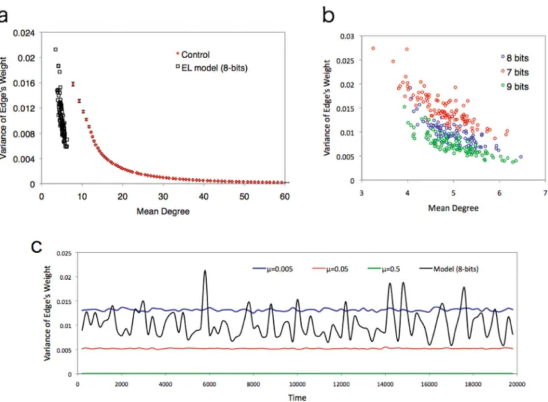
The trade-off relationship between these two factors (i.e. robustness and efficiency) was confirmed by using the control model for parameter tuning. Increasing the value ofμsuggests that the error increases for the fitness estimates of each individual. This tendency leads to the creation of a highly connected network because the error of fitness estimation increases the transitional possibility to many states. However, decreasing the value ofμreduces the error es-timation. Therefore, a low value ofμsuppresses false transitions due to errors. Instead, the weights of edges connected to correct states (corresponding to transitions to nodes near the tar-get) increase. This gives the network a high heterogeneous weight distribution.Fig 5Ashows the trade-off relationship between the degree of heterogeneity of the weights of the edges and the mean degree of the network (the parameter valuesμare taken from 0.005 to 0.1 for every 0.005 interval). This graph shows that the distribution of the weight of edges becomes almost uniform in highμareas, but not in lowμareas.
Compared with the control model, our model weakens the trade-off relationship between the edge weight distribution and mean degree. InFig 5A, wetake 200 samples from a certain instant of the EL model (Fig 5Bshows the trade-off relationship for 7, 8 and 9 bits. The same tendency was observed). Both values are distributed around the mean values. The variance from the mean values is much larger than the control model. This can be observed in the time series variance of the weights in one trial (Fig 5C). In the control model, the variance of edge weights is always much smaller than the EL model. This suggests that the network structure of each parameter value remains the same through the process of one trial. Compared with the control, the variance of the weights changes dynamically in the time series of the EL model. Taking into account the correlation relationship between the mean degree and weight variance, the network structure of the EL model is not stable but dynamic.
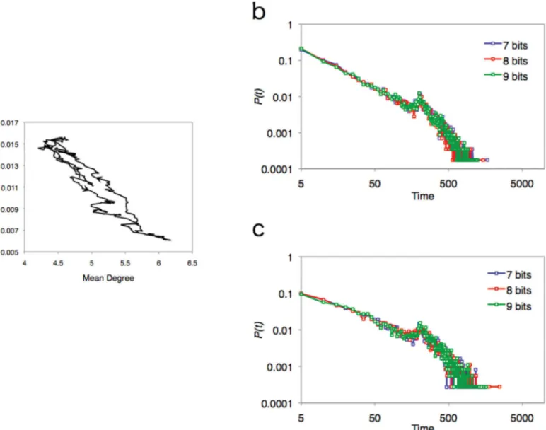
Next we examine the detail of the dynamics of the network structure of the EL model.Fig 6Ashows an example of the circle trajectory of the mean degree and the weight variance (other examples are listed inS3 Fig). We take each value at each interval such as 200–400, 201–401, 202–402, and so on. This graph indicates that the mean degree in this graph gradually increases as the weight variance of the network decreases, and vice versa. In other words, the network of the EL model tries to resolve the trade-off relationship itself by tuning the tensions between the two values. This tendency reflects the recurrence time of mean value of both measurements.
Fig 5Bshows that it takes a long time to get back to the mean values. In particular, the probabil-ity distribution of the recurrence time for the mean degree obeys a power law distribution (see
Discussion
The aim of this paper is to construct a non-ever-growing weighted network model by using fit-ness estimation, deduced from incomplete information. The main point of difference of our model from previous network studies is based on taking into account the internal dynamics of the network. Because of the constraint on the number of individuals (2nindividuals in total for nbits), the distribution of individuals is finite. Each state of an individual, which corresponds to a node, changes state in order to increase its own fitness but the number of nodes is always under 2nbecause the maximum possibility of states is 2nin a given network. This state change plays a role in the flow in this network. The network structure arises from exchanging this fi-nite resource in a certain interval.
By taking internal dynamics in account, we are able to examine the emergence of weighted networks from local interactions. First, we found that the structure of this network (i.e. the
Fig 5. Trade of relationship between the mean degree and variance of edge weights. (a)Trade-off relationship between the mean degree and variance of edge weights. Weights are renormalized at each dot. Red indicates the control model and black indicates the EL model. Bars around the red dots show the standard deviation.(b)Negative correlation between the mean degree and variance of edge weights for each case (Peason correlation test, 7-bits: N = 87,r =–0.832,p<10–16; 8-bits: N = 87,r=–0.800,p<10–16; 9-bits: N = 97,r=–0.823,p<10–16).(c)The time series of variance of edge weights for the control (μ=
0.005,μ= 0.05 andμ= 0.5) and EL model (8-bits). Each value oscillates with time. However, compared with EL model, the fluctuation of the variance of the edge weights is very small.
Fig 6. Trajectory and its recurrent time of mean degree and variance of edges weight. (a)Trajectory of data through 600 steps (8 bits). The arrow in the graph indicates the direction of the process. After forming a circular trajectory, the system finally returns to the initial point.(b)Probability distribution of the recurrent time for mean value of the mean degree. Colors correspond to number of bits (7 bits: blue, 8bits: red, 9 bit: green). The graph exhibits a power law distribution (7-bits:N= 119900, scaling exponentα= 1.39, AIC weights of power laww(p) = 1.00; 8-bits:N= 119800, scaling exponentα= 1.40, AIC weights of power laww(p) = 1.00; 9-bits:N= 119859, scaling exponentα= 1.40, AIC weights of power laww(p) = 1.00).(c)Probability distribution of recurrent time for mean value of the variance of edge weights. Colors correspond to the number of bits (7 bits: blue, 8bits: red, 9 bit: green). In contrast to the mean degree, the graph exhibits an exponential. (7-bits:N= 119900, scaling exponentλ= 0.031, AIC weights of power laww(e) = 1.00; 8-bits:N= 119800, scaling exponentλ= 0.031, AIC weights of power laww(e) = 1.00; 9-bits:N= 119859, scaling exponentλ= 0.031, AIC weights of power laww(e) = 1.00). doi:10.1371/journal.pone.0127284.g006
Table 3. Data for a scaling parameterαof the recurrent time of power law with AIC test.
Scaling Parameterα AIC weights:w(p)
7-bits 1.39 (N= 119900) 1.00
8-bits 1.40 (N= 119800) 1.00
9-bits 1.40 (N= 119859) 1.00
Scaling parameterαand Akaike information criterion (AIC) weights of power law fort−α.tmeans the
recurrence time for the mean degree of an EL net- work.
degree distribution) in the EL model exhibits an exponential distribution instead of a power law, and we also found an asymmetrical relationship between the in-degree and out-degree dis-tributions. These tendencies have been observed in real web networks [11]. Furthermore, we also confirmed that the weight distribution of edges obeys a power law which never depends on how the interval is taken. Although the slope of the power law is not stable, it is observed that power law behavior remains the same. All these results are good matches to previous stud-ies [11,16,18]. In this respect, our assumption of internal dynamics provides sufficient evi-dence to say that we have a new network modeling.
Finally, we comment on the trade-off relationship between the mean degree and variance of the weight distribution discussed in the last section. We note the practical meaning of the resolu-tion of the trade-off relaresolu-tionship in our model. In contrast to the control model, the network structure of the EL model dynamically changes with time. In particular, the mean degree and variance of the edge weights change in a highly correlated way. As we discussed, the high mean degree indicates the robustness of the network and the high variance of edge weights indicates the efficiency of the network. By tuning the balance between these two quantities, the network of the EL model always acts to resolve the trade-off relationship between efficiency and robustness.
We note structures that resemble ascendency theory in ecosystems. Ulanowicz measured the degree of network development by using the concept of ascendency [16,17]. Ascendency is defined as the product of total system throughput and average mutual information. From this definition, ascendency is high when the flows in a network are distributed heterogeneously. In addition, he also noted that decreasing ascendency indicates that the number of redundant pathways (more specifically, he consider other quantities such as dissipations, inputs, and out-puts) is large. This trade-off relationship between ascendency and redundant pathways corre-sponds to our discussion, that is, the trade-off relationship between the mean degree and variance of edge weights. Furthermore, Ulanowicz discusses the development of the network from the perspective of ascendency [17]. If the ascendency increases, then the degree of maturi-ty of the ecosystems increases. If the ascendency of the system were to decrease, it would indi-cate a reset (or death) of the system and a return to an initial state.
If we accept this argument, we can insist that the EL model exhibits growth and decline of the system which resolves the trade-off relationship between robustness and efficiency because the increasing ascendency corresponds to increasing variance of edge weights and decreasing ascendency (i.e. increasing redundancy) corresponds to increasing mean degree of the network. (We examined the relation between the mean degree and variance of edge weights for real eco-systems, and found a negative correlation. Pearson’s correlation test:N= 15,r= -0.73,
p= 0.0008. This value suggests that real networks also exhibit this trade-off relationship). Our network model is not purely dynamical, and also exhibits developmental cycles in certain time intervals. The network of the EL model gets old with time. After the network grows to a certain degree of maturity (heterogeneous structure), the network gradually decays (homogeneous structure) and prepares for the next cycle. The growing and decaying network in the EL model is one answer to the trade-off problem under the finite distribution of resources in developing systems.
Supporting Information
S1 Fig. Cumulative distribution of edge weights for a 200 step interval.Color correspond to parameter values (μ=0.5: blue,μ=0.05: red,μ=0.5: green). Power law like behavior is only observed with high parameter values.
S2 Fig. The relationship between R2value for the least squares method for a power law.The relationship between R2value for the least squares method for a power law for cumulative dis-tribution of edge weights and the parameterμ. The region of high parameter values (μ>0.7) and of low parameter values (μ<0.4) are poor fits to the power law behavior.
(EPS)
S3 Fig. Other examples of the trajectory of the EL model.Other examples of the trajectory of the EL model for 500 steps. All graphs show that the network of the EL model travels around the space and finally back to the initial state.
(EPS)
S1 Text. Basic concept of lattice theory, the algorithm of the control model and thair analy-sis.
(DOCX)
Author Contributions
Conceived and designed the experiments: TN YPG. Performed the experiments: TN. Analyzed the data: TN. Contributed reagents/materials/analysis tools: TN. Wrote the paper: TN.
References
1. Barabási AL, Albert R (1999) Emergence of Scaling in Random Networks. Science. 286, 509. PMID: 10521342
2. Albert R, Barabási AL (2002) Statistical Mechanics of Complex Networks. Rev. Mod. Phy. 47. 4. 3. Dorogovtsev SN (2009) Lectures on Complex Networks. Oxford Univ. Press.
4. Mandelbrot B (1953) An Informational Theory of the Statistical Structure of Languages. Communication Theory. Betterworth, London, p.486.
5. Li X, Chen G (2002) A Local-World Evolving Network Model. Physica A. 328. pp. 274–286.
6. Fan Z, Chen G, Ko KT (2004) Evolving Networks: From Topology to Dynamics. Journal of Control The-ory and Applications. 2. pp. 60–64.
7. Wen G, Zim D, Chen G, Geng X (2011) A Weighted Local-World Evolving Network Model with Aging Nodes Physica A. 390. pp. 4012–4026.
8. D’Souza RM, Krapivsky PL, Moore C (2007) The Power of Choice in Network Growth. Eur. Phys. J. B. 59. pp. 535–543.
9. Achliopatas D, D’Souza RM, Spencer J (2009) Explosive Percolation in Random Network. Science. 1453, 323.
10. Broder A, Kumar R, Maghoul F, Raghavan S, Stata R, Tomkins A, et al. (2002) Graph Structure in the Web. Comput. Netw. 33. pp. 309–320.
11. Meusel R, Vigna S, Bizer C, Lehmberg O (2014) Graph Structure in the Web Revisited: A Trick of The Heavy Tail. Proceedings of the Companion Publication of the 23rtd International Conference on World Wide Web Companion. pp. 427–432.
12. Granovetter M (1973) The Strength of Weak Ties. American Journal of Sociology. 78. 6. pp. 1360–380. 13. Granovetter M (1983) The Strength of Weak Ties: A Network Theory Revisited. Sociological Theory.
1. pp. 201–233.
14. Oka M, Ikegami T (2013) Exploring Default Mode and Information Flow on the Web. PLoS ONE 8(4): e60398. doi:10.1371/journal.pone.0060398PMID:23637749
15. Stouffer DB. (2010) Scaling from individuals to networks in food webs Functional Ecology, 24: 44–51. 16. Ulanowicz RE (1997) Ecology, The Ascendent Perspective. Colombia Univ. Press.
17. Ulanowicz RE (2002) The Balance Between Adaptability and Adaptation. Biosystems, 64: 13–22. PMID:11755484
19. Ito T, Tashiro K, Muta S, Ozawa R, Chiba T, Nishizawa M, et al. (2000) Toward a Protein-Protein Inter-action Map of the Budding Yeast: A Comprehensive System to Examine Two-Hybrid InterInter-actions in All Possible Combinations Between the Yeast Proteins. PNAS. 97, 1143–7. PMID:10655498
20. Rooney N, MacCann KS (2012) Integrating Food Web Diversity, Structure and Stability. Trends in Ecol-ogy and Evolution. 27. 1. pp.40–46. doi:10.1016/j.tree.2011.09.001PMID:21944861
21. Emmerson M, Yearsley JM (2004) Weak Interaction, Omnivory and Emergent Food-Web Properties. Proc. R. Soc. Lond. B. 271. pp. 397–405.
22. Banconi G, Barabási AL (2001) Competition and Multiscaling in Evolving Networks. Europhys. Lett. 54 (4). pp. 436–442.
23. Ergün G, Rodgers GJ (2002) Growing Random Networks with Fitness. Physica A. 303. pp. 261–272. 24. Vega YM, Vázquez-Prada M, Pacheco AF (2004) Fitness for Synchronization of Network Motifs.
Phy-sica A. 343. pp. 279–287.
25. Xu XJ, Peng XL, Zhang LJ, Yang GH (2010) Effect of Fitness on Mutual Selection in Network Evolution. Physics Procedia. 3. pp. 1795–1799.
26. Niizato T, Gunji YP (2013) Interactions Between Species and Environments From Incomplete Informa-tion. Biosystems. 111(3). pp. 145–155. doi:10.1016/j.biosystems.2012.12.003PMID:23333507 27. Clauset A, Shalizi CR, Newman ME (2009) Power-Law Distribution in Empirical Data. SIAM Review.
406. pp. 661–703.
28. Edwards AM, Phillips RA, Watkins NW, Freeman MP, Murphy EJ, Afanasyev V, et al. (2007) Revisiting Lévy Flight Search Patterns of Wandering Albatrosses, Bumblebees and Deer. Nature 449, 1044– 1049. PMID:17960243
29. Zheng D, Trimper S, Zheng B, Hui PM (2003) Weight Scale-Free Networks with Stochastic Weight As-signments. Phys. Rev. E. 71. 67. 040102. pp.1–4.
30. Barrat A, Barthélémy M, Vespignani A (2004) Modeling the Evolution of Weighted Networks. Phys. Rev. E. 70. 066149. pp.1–11.
31. Antal T, Krapivsky PL (2005) Weight-Driven Growing Networks. Phys. Rev. E. 71. 026103. pp.1–6. 32. Bianconi G (2005) Emergence of Weight-Topology Correlations in Complex Scale-Free Networks.
Europhys. Lett. 71(6). pp.1029–1035.
33. Tong J, Zhang Z, Dai R (2011) Weight Scale-Free Networks Induced by Group Preferential Mecha-nism. Physica A. 390. pp.1826–1833.