MASTER
MATHEMATICAL FINANCE
MASTER
’
S FINAL WORK
D
ISSERTATION
T
HE
L
OTKA
-V
OLTERRA
E
QUATIONS IN
F
INANCE AND
E
CONOMICS
M
AFALDA
O
LIVEIRA
M
ARTINS
B
ASTOS DE
A
LMEIDA
MASTER
MATHEMATICAL FINANCE
MASTER
’
S FINAL WORK
D
ISSERTATION
T
HE
L
OTKA
-V
OLTERRA
E
QUATIONS IN
F
INANCE AND
E
CONOMICS
M
AFALDA
O
LIVEIRA
M
ARTINS
B
ASTOS DE
A
LMEIDA
S
UPERVISOR
:
J
OÃO
L
OPES
D
IAS
Acknowledgments
Resumo
As equac¸ ˜oes de Lotka-Volterra, tamb ´em conhecidas por equac¸ ˜oes de predador-presa, s ˜ao um conjunto de equac¸ ˜oes diferencias n ˜ao-lineares constru´ıdas para descrever a relac¸ ˜ao din ˆamica entre esp ´ecies na natureza. No entanto, desde a sua publicac¸ ˜ao v ´arios autores t ˆem vindo a provar que estes sistemas din ˆamicos t ˆem diversas aplicac¸ ˜oes fora da ´area da biologia. Este trabalho tem como objetivo apro-fundar as poss´ıveis aplicac¸ ˜oes destas equac¸ ˜oes ao sistema banc ´ario e `a economia. Considerando o sistema banc ´ario, estudamos tr ˆes poss´ıveis sistemas din ˆamicos que podem descrever a relac¸ ˜ao entre o volume de dep ´ositos e empr ´estimos num banco. Tamb ´em apontamos as semelhanc¸as entre um sis-tema banc ´ario de tr ˆes n´ıveis e uma cadeia alimentar e estudamos a sua estabilidade. Olhando para as aplicac¸ ˜oes `a economia, comec¸amos por estudar o famoso modelo de Goodwin para ciclos de de-semprego e crescimento dos ordenados. Para terminar, apresentamos um par de equac¸ ˜oes predador-presa que descrevem a relac¸ ˜ao entre bens capitais e bens de consumo, e conclu´ımos que os ciclos econ ´omicos s ˜ao end ´ogenos, auto-sustent ´aveis e n ˜ao-lineares.
Abstract
The Lotka-Volterra equations, frequently referred to as predator-prey equations, are a set of non-linear differential equations constructed to describe the interaction dynamics between different species in na-ture. Yet, since their publication many authors have proved that the applications of these equations go way beyond mathematical biology. The present work focuses on their application to the banking system and to economics. Regarding the banking system, we study three dynamical systems that may describe the relationship between deposit and loan growth in a bank’s balance sheet. In addition, we look at the resemblance between a three level ecological food chain and a three level banking system, and study its stability. As for the applications to economics, we study the famous Goodwin’s model for the cyclic behavior of wages and employment. To finish our work we present a pair of predator-prey equations that model the dynamical relationship between consumption and capital goods, finding that economic cycles are endogenous, self-sustained and non-linear.
Contents
Acknowledgments . . . iii
Resumo . . . iv
Abstract . . . v
List of Figures . . . viii
1 Introduction 1 2 Literature Review 3 3 Theoretical Framework 5 3.1 The Predator-Prey Model . . . 5
3.2 General Lotka-Volterra Systems . . . 7
3.3 Competitive Lotka-Volterra Systems . . . 9
3.3.1 Two Species Dynamics . . . 9
3.3.2 N Species Dynamics . . . 12
3.4 Cooperative Lotka-Volterra Systems . . . 14
3.4.1 Two Species Dynamics . . . 14
3.4.2 N Species Dynamics . . . 16
4 Lotka-Volterra Equations in the Banking System 18 4.1 Deposit and Loan Growth . . . 18
4.1.1 A Simple Model . . . 19
4.1.2 A model with Michaelis-Menten Response . . . 20
4.1.3 A model with Reserve Requirement . . . 21
4.2 Three Level Banking System . . . 21
5 Lotka-Volterra Equations in Economics 24 5.1 Goodwin’s Model . . . 24
5.1.1 The Original Model . . . 24
5.1.2 A Revised Model . . . 27
5.1.3 An Improved Model . . . 29
6 Conclusions 34
List of Figures
3.1 Stability of the Predator-Prey Model. . . 6
3.2 Predator population without Prey . . . 7
3.3 Prey population without Predators . . . 7
3.4 Unidimentional Logistic Equations. . . 10
3.5 a12= 0.5anda21= 0.25 . . . 12
3.6 a12= 1.5anda21= 1.2. . . 12
3.7 a12= 0.5anda21= 2.1. . . 12
3.8 a12= 1.5anda21= 0.5. . . 12
3.9 a12= 0.5anda21= 0.25 . . . 15
3.10a12= 1.5anda21= 0.5. . . 15
3.11a12= 1.5anda21= 1.2. . . 15
3.12a12= 0.5anda21= 2.1. . . 15
4.1 Stability of the Simple Model for Deposit and Loan Growth. . . 19
4.2 Three Level Ecological System . . . 22
4.3 Three Level Banking System . . . 22
4.4 Solution of System (4.6) on the planex1= 0. . . 23
5.1 Weight FunctionG(s) =ae−as, a= 0.75.. . . . 29
Chapter 1
Introduction
The Lotka-Volterra equations, often referred to as the predator-prey equations, are first order non-linear differential equations that describe the dynamics of populations in systems where multiple species, with distinct characteristics, interact.
In the United States, 1925, Alfred Lotka proposed a model to describe a chemical reaction with oscil-lating concentrations. A year later, in Italy, the mathematician Vito Volterra, when trying to explain the observed increase in predator fish (that caused a decrease in prey fish) in the Adriatic Sea during World War I, independently arrived to the same set of equations proposed by Lotka. This model proposed by Lotka and Volterra is considered to be the simplest model for predator-prey interactions.
If we aim to study the populations’ dynamics in a single species environment, we should concentrate on factors such as the natural growth rate and the environment’s carrying capacity. Yet, if we aim for a more realistic approach we need to study interacting populations and remember that they affect each other’s growth rates. Interacting populations affect one another’s evolution, and predicting the result of their relationship is of high interest to understand how communities are organized and sustained.
Ever since the publication of the predator-prey population model, authors have used these equations not only in the study of ecological systems but also in other scientific areas. In the present work, we focus on the applications of the famous Lotka-Volterra equations to economics and to the banking system.
To start, in Chapter 2 we mention some of the most important studies presented throughout time regard-ing the Lotka-Volterra equations and their possible applications.
where species interact in a way that benefits one another, once again starting with the two-species case and extending the results to an environment ofnspecies.
In Chapter 4 we focus our attention in the applications of the Lotka-Volterra equations to the banking system. First, we present a dynamical system identical to the two-species predator-prey model that describes the relationship between deposit and loan growth inside the capital structure of a bank, as well as some other models constructed for the same porpoise but with different features. In the second part of this chapter we present a model that compares a three level banking system to a three species ecological food chain.
Chapter 2
Literature Review
The Lotka-Volterra equations for predator-prey models are very famous in mathematics as well as in bi-ology. The biologist Umberto D’Ancona suggested that the interactions between various animal species could be mathematically modeled, and this resulted in the publication of [1] and later [2] by the mathe-matician Vito Volterra. Among the several models proposed by Volterra there is the predator-prey case, the most famous one. Since Volterra did not know the work of Alfred J. Lotka, who had independently anticipated some of Volterra’s results in [3], these equations were named Lotka-Volterra equations.
There are many applications of the predator-prey model, including in Game Theory. For example, in 2010 Chen [4] proposed a model for predation behavior applied to Game Theory and concluded that the smaller predators tend to use a more passive strategy than large predators, and that preys always prefer an active strategy.
The derivation of dynamical models based on bank profit were first proposed in 2008 by Petersen and Shoeman [5], who analyzed the Return-on-Assets and the Return-on-Equity of a bank. Later that year, the economic aspects of the stochastic dynamics model of a bank’s assets and liabilities were presented on [6]. In 2012, Comes proposed a three dimensional dynamical model to describe the interaction be-tween levels of the banking system [7] and used the results on the work of Apreutesei [8][9] to study its stability. In 2013, the first dynamical system of deposit and loan volumes based on the Lotka-Volterra predator-prey dynamics [10] was presented, and in 2014 Sumarti, Nurfitriyana and Nurwenda studied the equilibria of this type of dynamical systems [11].
relaxing some of the original assumptions. On the other hand, Velupillai (1979) [17] and Flaschel (1984) [18] investigated the stability and other mathematical properties of the model; In addition, authors like Atkinson (1969) [19] and Harvie (2000) [20] have focused on verifying the model’s validity by testing it.
Chapter 3
Theoretical Framework
Lotka-Volterra systems of equations model the dynamics of n interacting species (and they can also be applied in the study of financial institutions and economic behavior) According to this model, the populations change through time according to a system of differential equations of the form
˙
xi=xi
ri+ n
X
j=1 aijxj
, i= 1, ..., n (3.1)
whereri∈RandA= (aij)is a matrix of real entries.
In this chapter we will start by studying a general predator-prey system of equations for two interacting species and some of its important features. Later, we will return to the general form of a Lotka-Volterra system and focus our attention on two specific types of interaction between species: competitive and cooperative. For each of these cases we analyze the two species model followed by a generalization to a system ofnspecies.
3.1
The Predator-Prey Model
In the early 90’s Volterra presented a model to describe the evolution of predator and prey fish popula-tions in the Adriatic Sea. He based his model in two assumppopula-tions: First, in the absence of predators the per capita growth rate of the prey population is constant and positive. Otherwise, it decreases linearly as function of the predator population; Second, in the absence of prey the per capita growth rate of the predator population is constant and negative. Otherwise, it increases linearly as a function of the prey population.
assumptions translate into
1
N dN
dt =a−bP
1
P dP
dt =cN −d
(3.2)
where a, b, c, d > 0 are constants and N(0), P(0)
= (N0, P0). Also, if we manipulate the previous equations we get
d dt
dlogN−cN+alogP−bP = 0. (3.3) Let us defineH :R+0 ×R
+
0 →Rsuch that
H(N, P) =dlogN−cN+alogP−bP.
It is easy to see that d
dtH(N, P) = 0i.eH is constant along the trajectories N(t), P(t)
. Since we aim to studyH(N, P)depending on the initial condition(N0, P0), we split the problem in two cases.
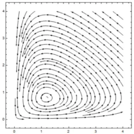
First, we assume that (N0, P0) ∈ R+×R+, so we have the guarantee thatH(N0, P0)is finite and all trajectories(N(t), P(t))evolve so thatH N(t), P(t)
=H(N0, P0). This happens becauseH(N, P)is a strictly concave function which implies that the orbits are periodic and that the function has a unique maximum where∇H = 0, i.e
(N, P) =d
c, a b
.
For the particular case where a = 2, b = 2.5, c = 2.3 andd = 2.7 the stability of the predator-prey system can be found in figure 3.1.
Figure 3.1: Stability of the Predator-Prey Model.
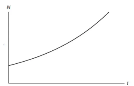
Second, we consider the possibility of either N0 or P0 being null, which allows us to obtain explicit solutions to the system in (3.1):
N0= 0 =⇒ N(t) = 0,P(t) =P0e−dt P0= 0 =⇒ N(t) =N0eat,P(t) = 0
Therefore, ast→ ∞, the solution exponentially approaches the origin along the lineN = 0and expo-nentially goes to infinity along the lineP = 0. Figure 3.2 shows the population of the predators across time in the absence of preys and figure 3.3 shows the evolution of the prey population in the absence of their predators.
Figure 3.2: Predator population without Prey Figure 3.3: Prey population without Predators
After studying these two cases we can conclude that the model makes basic sense, since regardless of the choice of initial condition we obtain non-negative populations. At this point we find it useful to introduce Volterra’s Principle: Suppose thatN0 > 0andP0 >0. IfT is the period of the closed orbit through(N0, P0)then the averages ofP(t)andN(t)overT are given respectively by
1
T
Z T
0
P(t)dt=a
b
1
T
Z T
0
N(t)dt=d
c.
(3.5)
Another important feature concerning the predator-prey equations is that system (3.2) is Hamiltonian, withH as its Hamiltonian function. Introducing the canonical coordinatesp= logN andq= logP we get
H(N, P) =h(p, q) =dp−cep+aq−beq
and the Lotka-Volterra equations are transformed into the canonical equations of Hamilton:
dp dt =
1
N dN
dt =a−bP =a−be
q= dh
dq dq
dt =
1
P dP
dt =cN−d=ce
p−d=−dh
dp.
(3.6)
3.2
General Lotka-Volterra Systems
Theorem 1 (Picard’s existence theorem) Given an open setU ⊆Rn, a functionf : U → Rn that is locally Lipshitz inx∈U and a pointx0 ∈U, the differential equationx˙ =f(x)withx(t0) =x0 has an unique solutionx:I→U on some open intervalIcontainingt0.
Definition 1We say that the vector fieldf :U →Rngenerates the flowϕ
t:U →Uwhereϕt(x) =φ(x, t)
forx∈U andt∈I= (a, b)⊆Rfor somea, b∈Rif dφ(x, t)
dt
t=τ
=f φ(x, τ)
, ∀x∈U, τ ∈I.
Definition 2 (Steady State)A Steady state ofx˙ =f(x)is a pointx∈U for whichf(x) = 0.
Definition 3 (Forward invariant set)A setS⊆U is a forward invariant set forϕtif wheneverx∈S we
haveϕt(x)∈Sfor allt≥0.
Definition 4 (Omega limit point) A point p ∈ U is an omega limit point of x ∈ U if there are points ϕt1(x), ϕt2(x), ...on the orbit ofxsuch thattk→+∞andϕtk →pask→ ∞.
Definition 5 (Alpha limit point) A point p ∈ U is an alpha limit point of x ∈ U if there are points ϕt1(x), ϕt2(x), ...on the orbit ofxsuch thattk→ −∞andϕtk →pask→ ∞.
Recall that the general Lotka-Volterra model is of the form (3.1). Applying Picard’s existence theo-rem we conclude local existence and uniqueness of solutions for any initial condition. Suppose that x(0) = (x01, x02, ..., x0n) hasx0k = 0 fork ∈ J ⊂ {1, ..., n} so that some species are initially absent.
Then, uniqueness of solution tells us that these species are absent for allt.
Theorem 2 For a model of the form (3.1) the coordinate axes and the subspaces spanned by them, and(R+)n, are all forward invariant. In simpler words, populations that start negative remain
non-negative throughout finite time.
Theorem 3 (Interior steady states)There exists an interior steady statep∈(R+)n if and only if (3.1)
has omega or alpha limit points in(R+)n.
Proof: The proof can be found in [24].
Theorem 4 (Time averages) Suppose thatx(t)is a periodic orbit of (3.1) of periodT. If (3.1) has a unique interior steady statex∗∈(R+)n, then
1
T
Z T
0
Proof:
˙
xi=xi
ri+ n
X
j=1 aijxj
=⇒ 1
T
Z T
0
˙
xi(t)
xi(t)
dt= 1
T
Z T
0
ri+ Ax(t)
idt
=⇒ 1
T
logx(T)−logx(0)=r+
"
A1 T
Z T
0
x(t)dt
#
=⇒ 0 =A−1r+ 1
T
Z T
0
x(t)dt
=⇒ 1
T
Z T
0
x(t)dt=−A−1r
=⇒ 1
T
Z T
0
x(t)dt=x∗
(3.7)
3.3
Competitive Lotka-Volterra Systems
The competitive Lotka-Volterra equations describe a model for the population dynamics of species com-peting for some common resource. These equations cover both competition between members of the same species and competition between members of different species. While in the predator-prey equa-tions the population model is exponential, in the competitive case it follows the logistic equaequa-tions we will introduce throughout this section.
3.3.1
Two Species Dynamics
When considering an environment with a single population, the logistic equation is
dN dt =ρN
1−N
K
, (3.8)
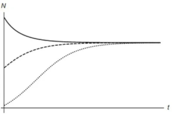
whereN(t)is the size of the population at timet,ρis the per-capita growth rate andKis the maximum population density that the environment can carry, often referred to as the environmental carrying ca-pacity. The quadratic term of the equation represents the competition between members of the same species for a common resource and we call this intraspecific competition. The previously presented logistic equation has an explicit solution of the form
N(t) = N N0
0
K + 1− N0
K
e−ρt
which implies that ast→ ∞the population approaches its carrying, regardless the initial conditionN0. This tendency is illustrated in figure 3.4.
Figure 3.4: Unidimentional Logistic Equations.
of each species and both with an extra term representing the interspecific competition. This new model writes
dN1
dt =ρ1N1
1−N1
K1
−c1N2 dN2
dt =ρ2N2
1−N2
K2 −c2N1
(3.9)
wherec1, c2>0are the relative sizes that measure the aggressiveness of the competition between the two species. Aiming to study the solution of (3.9) we defineN1(0) =N10andN2(0) =N20, and split the problem in two cases.
First, we consider the case where either N10 or N20 is null. Using the solution for the single-species logistic equation, we conclude that in the absence of one species the other approaches exponentially its carrying capacity:
N10= 0 =⇒ N1(t) = 0,N2(t) = N20 N20
K + 1− N20
K
e−ρ2t
N20= 0 =⇒ N1(t) = N10 N10
K + 1− N10
K
e−ρ1t
,N2(t) = 0.
(3.10)
In the second case we assume bothN10andN20to be positive numbers. For simplicity of calculations we set new variables and parameters:u1= N1
K1;u2=
N2
K2;a12=c1K2;a21=c2K1;τ=ρ1t;ρ=
ρ1
ρ2. This
gives us a new set of equations with less parameters but same behavior as before:
du1
dτ =u1(1−u1−a12u2) du2
dτ =ρu2(1−u2−a21u1).
(3.11)
Note that the Jacobian of this system has sign structure
J =
∗ ≤0
≤0 ∗
more specifically, it is of the form
J =
1−2u1−a12u2 −a12u1
−ρa21 ρ(1−2u2−a21u1)
Our first step in studying (3.11) is finding the lines on whichu1˙ = 0andu2˙ = 0: u1= 0 ∨ 1−u1−a12u2= 0
u2= 0 ∨ 1−u2−a21u1= 0
(3.12)
and these conditions allow us to identify the equilibrium points of the system:
(0,0); (1,0); (0,1); P = 1−a12 1−a12a21,
1−a21
1−a12a21
.
The second step in studying (3.11) is to assure that the coordinates of the steady points we found do not contradict the non-negativity of the populations. The first three points present no problem since they are in the non-negative part of the coordinate axes regardless the choice of parameters. As forP, we need to look at the values ofa12anda21.
The third and final step consists in studying the stability of each of the equilibrium points of (3.11), depending on the choice of parameters:
• Case 1:a12, a21<1;
The steady state P is stable, (0,0) is unstable and both (1,0) and (0,1) are saddles. These small values fora12anda21represent a competition that is not too aggressive and results in both populations coexisting in an equilibrium and never reaching their respective carrying capacities, as it shows in figure 3.5.
• Case 2:a12, a21>1;
The steady states P and (0,0) are unstable nodes. Here, both (1,0) and (0,1) are stable and there is an invisible line that separates the plane in two regions. Above this line all trajectories go to(1,0), otherwise they are attracted to(0,1). Orbits that start in the separation line converge to the unstable nodeP. The higher values fora12anda21considered in this case represent strong interspecific competition which leads to one of the species eventually winning and the other being driven to extinction. The winner depends upon which has the starting advantage, as is shown on figure 3.6.
• Case 3:a12<1, a21>1;
In this case there is no interior steady stateP. The states(0,0)and(0,1)are unstable but(1,0)is stable and attracts all trajectories. Here we havea12, which represents how competitive species2
• Case 4:a12>1, a21<1;
Once again there is no interior steady stateP. Here(0,0)and(1,0)are unstable but(0,1)is stable and all interior trajectories go to this state. In this case species2is more competitive and figure 3.8 shows that this leads to the extinction of species1.
Figure 3.5: a12= 0.5anda21= 0.25 Figure 3.6: a12= 1.5anda21= 1.2
Figure 3.7:a12= 0.5anda21= 2.1 Figure 3.8: a12= 1.5anda21= 0.5
3.3.2
N Species Dynamics
Now we consider the Lotka-Volterra system
˙
xi=xi
ri− n
X
j=1 aijxj
, i= 1, ..., n (3.13)
under the special condition thataij >0for alli, j ∈ {1, ..., n}. This means that each species competes
with all other species and that individuals of the same species compete with each other. Note that if ri ≤ 0, even in the absence of competitors, species iwould lead itself to extinction. For that reason,
sign structure: J = ∗ ≤ ≤ . . . ≤ ≤ ∗ ≤ . . . ≤ .. . ... ... . .. ... ≤ ≤ ≤ . . . ∗
Lemma 1Sinceaij>0andri>0, all orbits of (3.13) are bounded.
Proof: We know that(R+0)nis invariant. Also, from
˙
xi=xi
ri+ n
X
j=1 aijxj
=⇒ rixi−xi n
X
j=1 aijxj
=⇒ x˙i≤rixi−aiix2i
=⇒ x˙i<0ifxi>
ri
aii
(3.14)
we can conclude that for eachi= 1, ..., nthe populationxiis bounded.
Lemma 2Under the assumption that
rj ajj < ri
aij, if1≤i < j ≤n
rj
ajj >
ri
aij, ifn≥i > j≥1
the competitive system (3.13) has no interior steady state.
Proof: According to [24], ifx∗is an interior steady state then:
ai1 ri
x∗1+ ai2
ri
x∗2+...+ ain
ri
x∗n= 1, i= 1, ..., n.
Therefore, for eachiwe can write
a11 r1 −
ai1 ri
x∗1+
a12 r1 −
ai2 ri
x∗2+...+
a1n
r1 −
ain
ri
x∗n= 0
and if we specifyi=nwe get
a11 r1 −
an1 rn
x∗1+
a12 r1 −
an2 rn
x∗2+...+
a1n
r1 −
ann
rn
x∗n = 0.
From the second equation on Lemma 2, we know that the onlyx∗that verifies this equality is the trivial
equilibriumx∗= 0. Therefore, the system (3.12) has no interior steady states.
Theorem 5 (Extinction in competitive Lotka-Volterra)Under the assumptions on Lemma 2, r1
a11,0, ...,0
3.4
Cooperative Lotka-Volterra Systems
In contrast with the previous section, here we study the dynamics of an environment where species cooperate with each other but elements of the same species still compete for the same resources. Cooperative Lotka-Volterra logistic equations model the density of a pool of species taking into account that they work together for common benefit. This phenomenon, when considering only two species, is called mutualism.
3.4.1
Two Species Dynamics
Mutualism is the way two organisms of different species exist in a relationship where each individual benefits from the activity of the other. It contrasts with interspecific competition, where one species benefit at the ”expense” of the other. The logistic equations for the case of mutualism are similar to the ones in the case of competition (3.9), the only difference being the sign of the interaction terms. For this type of problem we have
dN1
dt =ρ1N1
1−N1
K1 +c1N2
dN2
dt =ρ2N2
1−N2
K2 +c2N1
.
(3.15)
Allowing one species to start with null population implies that it will remain null for all time, which leads us to the solution in (3.10) once again. On the other hand, when considering initial populationsN10and N20positive we introduce the same parameters and variables as we did when simplifying the competitive two-species dynamics and obtain
du1
dτ =u1(1−u1+a12u2) du2
dτ =ρu2(1−u2+a21u1)
(3.16)
with steady states
(0,0); (1,0); (0,1); P = 1 +a12 1−a12a21,
1 +a21
1−a12a21
.
Note thatP only exists whena12a21 <1, since we need to guarantee the non-negativity of the popula-tions. The Jacobian of this system has sign structure
J =
∗ ≥0
≥0 ∗
more specifically
J =
1−2u1+a12u2 a12u1 ρu2a21 ρ(1−2u2+a21u1)
To study the stability of the two species cooperative equilibrium we consider the following cases:
• Case 1:a12a21<1;
There are four steady states and all trajectories converge to the stable nodeP, the only one which does not lie on the coordinate axes. This behavior holds regardless of the choice ofa12anda21, which is illustrated in figures 3.9 and 3.10.
• Case 2:a12a21>1;
There are only three steady states : (0,0),(0,1)and(1,0). In the absence of an interior stateP all orbits diverge to infinity as can be observed in figures 3.11 and 3.12. This behavior holds for all values ofa12anda21.
Figure 3.9: a12= 0.5anda21= 0.25 Figure 3.10:a12= 1.5anda21= 0.5
3.4.2
N Species Dynamics
To study Lotka-Volterra cooperative systems for the interaction ofnspecies, we simply write
˙
xi=xi
ri+ n
X
j=1 aijxj
, i= 1, ..., n (3.17)
whereri ∈ R,A = (aij)is a matrix of real entries and aij ≥0wheni 6=j. This is very similar to the
general case, but with the restriction that the term representing interspecific interaction is non-negative due to each species benefiting from the existence of the others. Therefore, the interaction matrixAhas off-diagonal elements greater or equal than zero and the Jacobian of (3.17) has the sign structure :
J = ∗ ≥ ≥ . . . ≥ ≥ ∗ ≥ . . . ≥ .. . ... ... . .. ... ≥ ≥ ≥ . . . ∗
Definition 6 (Cooperative matrix)We say that any realn×nmatrix with the previous sign structure is cooperative.
Definition 7 (Negatively diagonally dominant) A matrixA is negatively diagonally dominant if there existsd∈Rnsuch thatdi>0andaiidi+Pi6=j|aijdj|<0for alli= 1, ..., n.WhenAis cooperative, this
translates to(Ad)i<0for alli= 1, ..., n.
Definition 8 (Stable Matrix)A square matrixAis said to be stable if every eigenvalue ofAhas strictly negative real part.
Lemma 3LetAbe a cooperative matrix. ThenAis stable if and only if it is negatively diagonally domi-nant.
Proof: First, let us assume thatAis a stable cooperative matrix. Then, for a sufficiently large positivec we get a non-negative matrix of the formB =A+cI. Therefore, by the Perron-Frobenius theorem we can guarantee the existence of a spectral radiusλ=ρ(B)≥0andv >0such thatBv =λv =ρ(B)v, which means Av = (ρ(B)−c)v whereρ(B) < c(because we are assuming Ato be a stable matrix). Then, the series
A−1=−1
c
I+1
cB+
1
c2B 2+
...
converges and all tranches of the sum are≤0. If we setd=−A−1(1, ...,1)T, it is easy to see thatd >0
and thatAd=−(1, ...,1)T <0meaning thatAis negatively diagonally dominant.
Awith an eigenvectorxto the right. Also, letyi = xdii and we choosemsuch that|ym|=maxi|yi|>0.
Then,
λdiyi= n
X
j=1 aijdjyj
and in particular, takingi=mand dividing byymwe can write
λdm=dmamm+ n
X
j6=m
djamj
yj
ym
.
Since by hypothesis we have that
aiidi+
X
i6=j
|aijdj|<0
we can conclude
|λdm−dmamm| ≤ n
X
j6=m
djamj
yi ym ≤ n X
j6=m
djamj<−dmamm
which means that|λ−amm|<−amm, implying that for every choice ofλit has negative real part.
There-fore, the cooperative matrixAis stable.
Corollary 1 If A is cooperative andri > 0 for all i = 1, ..., nthenAx+r = 0 has an unique interior
solutionx∈(R+)nif and only ifAis stable.
Definition 9 (Lyapunov stability)A steady statex∗is said to be Lyapunov stable if for anyǫ >0there isδ >0such that for allx0 with|x∗−x0|< δwe have|ϕ(x0, t)−x∗|< ǫfor allt≥0. A steady state is said to be unstable if it is not Lyapunov stable.
Definition 10 (Asymptotic stability)A steady statex∗ is said to be locally asymptotically stable if it is
Lyapunov stable and there isρ >0such that for allx0with|x∗−x0|< ρwe have|ϕ(x0, t)−x∗|< ǫfor
allt≥0.
Theorem 6 (Global convergence for cooperative Lotka-Volterra) Suppose that the system (3.15), with each ri >0, has an unique interior steady statex∗ and thatA has non-negative off diagonal
el-ements. Then, x∗ is globally asymptotically stable on (R+)n and all (boundary) orbits are uniformly
bounded ast→ ∞.
Chapter 4
Lotka-Volterra Equations in the
Banking System
Banking regulations can be governmental and non-governmental and they are managed with specific requirements, restraints and guidance. This guarantees transparency between banks and the institutions with whom they work. Financial institutions have high influence on the economy and their behavior can have great impact regarding global instability.
4.1
Deposit and Loan Growth
Banks use the deposits made by clients as funds to administer loans and they benefit from the differ-ence between the interest rates agreed to on the deposits and loans. For this reason, it is important to understand the interaction between deposit and loan volume.
Sumarti, Nurfitriyana and Nurwenda (2014) [10] proposed a dynamical system for deposits and loan volumes in a bank using the predator-prey equations. They argued that, as the existence of predators depends on the existence of prey, the existence of loans depends on the existence of deposits since the bank’s loan volume is defined as a portion of its deposit volume.
In a bank’s balance we find its liabilities, assets and equity. The bank’s liabilities are the obligations that must be paid in the future, and the bank’s assets consist on the investments and resources expected to give income in the future. The bank’s equity is calculated by making the difference between its assets and liabilities.
The main liabilities of a bank are the deposits made by costumers(D) while its main assets are the loans(L), the primary reserve(R1)and the secondary reserve(R2). Their interaction is described by
which means that there is a relationship between the volume of loans and reserves, and the deposits. Next, we will explore this dependence starting by comparing it with a predator-prey interaction where the loans and reserves represent the predators and the deposits represent the prey.
4.1.1
A Simple Model
The model proposed in [10] for the interaction between loan and deposit volumes based on the Lotka-Volterra predator-prey equations writes:
1
D dD
dt =α−pL
1
L dL
dt =pD−β
(4.2)
whereαis the interest rate of the deposit andβ is the interest rate of the loan, which makes both pa-rameters positive constants. Furthermore, p is the maximum mixture rate between deposit and loan volumes. Looking at this system we can observe that an increase inαwill cause and increase in deposit volume, as an increase inβ will cause a decrease in loan volume. On the other hand an increase on pDL, which represents the mixture between the deposit and loan volumes, will cause a decrease in the growth of deposit volume and an increase in loan volume growth though time.
System (4.2) has three equilibrium points:
P1= (0,0); P2=β
p, α p
;
In the context of our problem,P1is a saddle point andP2is a stable node ifα < β, i.e the interest rate on the deposit is lower than the interest rate of the loan, which makes sense according to reality.
Assumingα= 0.3,β = 0.5andp= 20the stability of this model for the dynamics of deposit and loan growth is illustrated in figure 4.1
Note that, just like the predator-prey system in (3.2), this model can be written in Hamiltonian coor-dinates. Considering m = logD and n = logL and denoting byH the Hamiltonian function we can write
H(D, L) =h(m, n) =βm−pem+αn−pen. Then, the equations in (4.2) become
dm dt =
1
D dD
dt =α−pL=α−pe
n= dh
dn dn dt = 1 L dL
dt =pD−β =pe
m−β =−dh
dm.
(4.3)
which proves that the system is Hamiltonian.
4.1.2
A model with Michaelis-Menten Response
Kar (2005) [25] proposed a model on this subject based on a study presented by Michaelis and Menten (1913) [26] concerning the saturation curve for enzyme reactions. Kar’s model was based on the as-sumption that the deposit volume is limited and the loan volume approaches a constant as the deposits increase. Note that, under these conditions, the model no longer follows a Lotka-Volterra system of equations:
dD dt =αD
1−D
k
− pDL
1 +bD dL
dt = pDL
1 +bD−βL
(4.4)
whereα, β, k, pandbare positive constants. Furthermore,kis the carrying capacity of the deposit vol-ume and pb is the maximum portion of the deposits that can be invested in the loans.
This model has three equilibrium points:
P1′= (0,0); P2′= (k,0); P3′ =
β p−bβ,
α pk−(1 +bk)β
k(bβ−p)2
;
HereP′
1is once again a saddle point andP2′ is stable ifβ= 1+pkbk, i.e the interest rate of the loan will rise
with an increase in the deposit’s carrying capacityk. Furthermore,P′
3only exists ifβ6= pb and is a stable
equilibrium if
α
2pk(bβ−p) (bk+ 1)bβ
2+ (1− bk)pβ
<0
and
4.1.3
A model with Reserve Requirement
Kar (2005) [25] also proposed a model including reserve requirements, i.e requirements regarding the amount of cash a bank must hold in reserve considering the deposits made by customers. This money must be in the bank’s vaults or at a Federal Reserve bank. If we considermDthe protected reserve, the model is of the form
dD dt =αD
1−D
k
− p(1−m)DL
1 +b(1−m)D dL
dt =
p(1−m)DL
1 +b(1−m)D −βL
(4.5)
with equilibrium points:
P′′
1 = (0,0); P2′′= (k,0); P3′′=
β
(1−m)(p−bβ),
(bk(1−m)−1)β+ (1−m)pk
α k(1−m)2(bβ−p)2
;
As in the previous modelsP′′
1 is a saddle point. On the other hand,P2′′is a stable equilibrium as long as we guarantee that, forα <1
β > k(1−m)p
1 +k(1−m)b. Furthermore,P3′′will be stable if
α −(1−m)b2k−b
β2+ (1−m)pbk−p
β
2(1−m)pk(bβ+p) <0
and
β < p (1−m)bk−1
b (1−m)bk+ 1.
4.2
Three Level Banking System
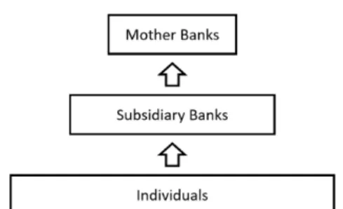
Thompson (2011) [27] argued that the financial system behaves like an ecological network in the fol-lowing way: ”Considering a three level food chain in ecological systems, we have biomass transfer from Herbivorous to Carnivorous and from plants to Herbivorous. On the other hand, in a financial system we have capital transfer from Mother Bank to Subsidiary Bank, and from Subsidiary Bank to Individuals or Companies.” A subsidiary bank is a type of foreign bank that is located in a country but is owned by a foreign mother bank. Subsidiary banks are regulated by their mother banks and at the same time have to perform under the rules of the host country.
Figure 4.2: Three Level Ecological System Figure 4.3: Three Level Banking System
dynamics:
˙
x1(t) =x1(t)(a1−b1x2(t) +c1x3(t)) ˙
x2(t) =x2(t)(−a2+b2x1(t)) ˙
x3(t) =x3(t)(a3−b3x1(t))
(4.6)
where ai, bi, ci > 0, i ∈ {1,2,3}. This system represents a three-level banking system where a top
predator Mother Bank ”feeds” on a intermediate consumer Subsidiary Bank , which ”feeds” on the In-dividuals that use its services. Furthermore, from Haimovici (1980) [28] and Apreutesei (2006) [9] we know that for every initial solution(x1(0), x2(0), x3(0))system (4.6) has an unique solution which is con-tinuous inR+0.
To study system (4.6) we start by solving each planar system in its respective coordinate plane. First, we notice that in the absence of mother banks (x2 = 0) the equations are reduced to a two-species predator prey model similar to the one studied in Section 3.1. In this case, we have closed orbits around the equilibrium a1
b1,
a3
b3,0
for all possible values of the parameters.
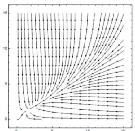
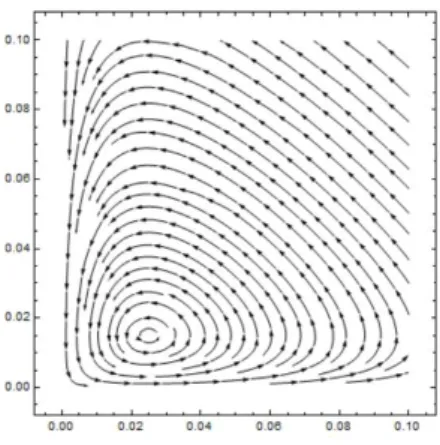
When considering the solution of (4.6) on the planex1= 0(when the subsidiary banks are absent from the system) we arrive to the system
˙
x1(t) = 0
˙
x2(t) =−a2x2
˙
x3(t) =a3x3
(4.7)
The equationx˙2(t) = −a2x2 implies thatx2(t)→0exponentially ast→ ∞, whilex˙3(t) =a3x3 means that x3(t) → ∞ exponentially ast → ∞. The behavior of the three level system in the absence of subsidiary banks is illustrated in figure 4.4, for the particular case wherea2, a3= 1.
missing from the equations(x3= 0), the system we need to solve becomes
˙
x1(t) =x1(−a1−c1x2) ˙
x2(t) =x2(−a2+b2x1) ˙
x3(t) = 0
(4.8)
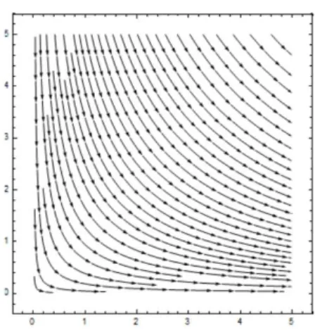
Looking at system (4.8), we can easily see that x1˙ ≤ −a1x1. This means that, as t grows to infinity, x1(t)will become null causingx2(t)to exponentially decay to zero. This tendency makes sense when we think of the three level banking system: in the absence of clients for the subsidiary banks, they will disappear since there is no demand for their services and that will cause the mother banks to also go extinct.
Figure 4.4: Solution of System (4.6) on the planex1= 0.
When studying the equilibrium of system (4.6), we first need to find the steady states by solving
˙
x1(t) = 0 ˙
x2(t) = 0 ˙
x3(t) = 0.
(4.9)
In the context of our problem, we find two equilibrium points:
P1= (0,0,0); P2=a2
b2, a1 b1,0
;
Next, to find the stability of this steady states, we compute the Jacobian of (4.6):
J =
a1−b1x2+c1x3 −b1x1 c1x1 b2x2 −a2+b2x1 0
−b3x3 0 a3−b3x1
Chapter 5
Lotka-Volterra Equations in
Economics
5.1
Goodwin’s Model
The behavior of economic systems has been described in three different ways in the literature. The first models considered the markets to be in a stable equilibrium, i.e even with random shocks the equilib-rium is always be restored. Later in time, models started to be constructed based on the assumption that growth is cyclical and its equilibrium is affected by past changes. More recently, with the arrival of modern statistical methods, economists found that random shocks create what features chaotic behav-ior: economic relations resemble white noise and economic motion is random.
Goodwin (1967) [13] presented a model describing the dynamic relationship between wages and em-ployment. Later on, this model was improved so it would incorporate the three behaviors of economic systems mentioned before: The economy would have stable wages and employment but small pertur-bations could lead cycles. Furthermore, a drastic change would cause the economy exhibit chaotic behaviour.
Throughout this section we will study Goodwin’s original model as well as some of its shortfalls, and to finish we will present an improved model that incorporates some important features missing in the original one.
5.1.1
The Original Model
profits. With more profit more workers will be hired causing a rise in employment levels and so a cycle arises.
These cycles are not the same as business cycles but they are related, since a recession can affect the employment cycle and,contrarily, changes in wages can cause a recession. Goodwin’s main goal with his study is to understand the cyclical behavior of employment, using the predator-prey equations to dynamically model income distribution and employment levels.
Goodwin’s model has its origin in an idea in Marx (1887) [29]. Marx believed that ”capitalism’s alternate ups and downs are a result of the dynamic interaction between profits, wages and employment”. To mathematically express this variations, Goodwin used the predator-prey equations and wrote his model based on the following assumptions:
Assumption 1:Both technological progress and growth in labor force are constant.
Assumption 2:There are only two factors of production (labor and capital).
Assumption 3:All quantities mentioned are real and net.
Assumption 4:All wages are consumed and all profits are saved and invested.
Assumption 5:The ratio between capital and output is constant.
Assumption 6:The real wage rate rises in the neighborhood of full employment.
Constant technological progress means growth in labor productivity of the form
a=a0eαt, α >0
whereais the labor productivity that grows at a constant rateα. On the other hand, assuming constant growth in labor force we can write
n=n0eβt, β >0
wherenrepresents the labor force growing at a constant rateβ. Also, denoting askthe capital and as qthe output, we obtain a constant capital-output ratio of
σ= k
q.
If we considerwthe wage rate, then the worker’s share of output will be given by
u=w
a
is equal to the profit and therefore
˙
k= (1−u)q.
Through some easy computations we find that the growth rate of capital over time is of the form
˙
k k =
(1−u)
σ
and since we have a fixed capital-output ratio the growth rate of output over time will be the same:
˙
q q =
(1−u)
σ .
At this point it makes sense to consider the employment as
l= q
a
and after some manipulation of the formulas we find that the change in employment over time is of the form
˙
l l =
(1−u)
σ −α.
The real employment rate is calculated by dividing employment by labor force
v= l
n
implying that the growth rate of real employment over time changes according to
˙
v v =
(1−u)
σ −(α+β). (5.1) As was mentioned before, Goodwin assumes that the real wage rate rises in the neighborhood of full employment. Therefore, we can describe the wage growth as
˙
w
w =ρv−γ and since the real wage rate is
u=w
a we finally obtain
˙
u
u =−(α+γ) +ρv. (5.2) Equations (5.1) and (5.2) together describe Goodwin’s employment-wage cycle model:
˙
v=h 1
σ−(α+β)
−u σ i v ˙ u=
−(α+γ) +ρv
u.
Goodwin arrived to a Lotka-Volterra predator-prey model of the form
˙
v= (η1−θ1u)v
˙
u= (−η2+θ2v)u
(5.4)
where
η1= 1
σ −(α+β) η2=α+γ
(5.5)
and
θ1= 1
σ θ2=ρ.
(5.6)
In the original predator-prey system we identify the predator and the prey by the fact that the predator population grows faster with an increase of prey population, while the prey population grows faster with a decrease of predator population. Looking at (5.4) it is clear that the employmentvrepresents the prey and the wagesuthe predators of this system.
We already know from the previous chapter that, in the presence of both species, the predator-prey model’s solution is a family of closed cycles with a common equilibrium point. For the system in (5.4) that point is
(v∗, u∗) =η2
θ2, η1 θ1
.
Using the original parameters, we can write the center of the economic model as
(v∗, u∗) =
(
α+γ)
ρ ,1−(α+β)σ
. (5.7)
5.1.2
A Revised Model
Goodwin’s model has some shortfalls, some of them even pointed out by Goodwin himself in his later work.
Unlimited Growth
The first problem with this model arises when we look at (5.4) and see that, in the absence of wagesu, the employment rate is given by
v=v0eη1t
workers are unlikely to be as productive as employed workers. Furthermore, labor market downsizing often excludes the less trained workers first, as an upsizing may lead to the acceptance of who is available regardless their training and skills. To make this model more realistic, one should consider a logistic saturation so that atu= 0we have
˙
v=η11− v
K
v.
In this model, we should considerK= 1, since the employment rate can’t be bigger than100%. Including this feature, the model would write:
˙
v=η1(1−v)v−θ1vu
˙
u= (−η2+θ2v)u
(5.8)
Wages and Employment
The second problem with Goodwin’s original model is the reaction of wages to employment, since any changes in wages as a result of changes in employment cannot be instantaneous as they are assumed to be. Wage contracts planed ahead and usually not don’t into account future demand for labor, causing a delay in the reaction of wages to employment. This delay can be introduced in (5.8) by replacing in the second equation
v=
Z t
0
v(τ)G(t−τ)dτ whereGis a non negative integrable weight function that verifies
Z t
−∞
G(t−τ)dτ =
Z ∞
t
G(s)ds= 1.
Therefore, the way wages depend on the past employment levels can be set according to the choice of functionG. With this modification, the new model writes
˙
v=η1(1−v)v−θ1vu
˙
u=−η2u+θ2u
Z t
0
v(τ)G(t−τ)dτ.
(5.9)
Structural Instability
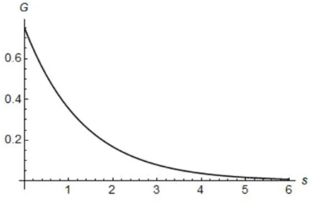
The structural instability of Goodwin’s model is considered to be its worst fault. This instabililty comes from the fact that small changes in the initial condition(v0, u0)may lead to a much different behavior of solutions. Cushing (1977) [30] and MacDonald (1977) [31] managed to stabilize the solutions by choosing as weight function
This means that these authors considered that employers take into account changes in the company’s profits before making the wage contracts. Due to the constant capital-output ratio and the fact that output is strongly connected to employment, employers discount past employment levels usingaas a discount rate. Using this weight function, the authors guarantee that the furthest in the past an employment level is the less it affects the wages. Furthermore, if we consider a time periodslarge enough the influence becomes practically null, as can be observed in figure 5.1.
Figure 5.1: Weight FunctionG(s) =ae−as, a= 0.75.
These authors wrote a variation of system (5.9) without structural instability:
˙
v=η1(1−v)v−θ1vu
˙
u=−η2u+θ2u
Z t
0
v(τ)ae−a(t−τ)dτ. (5.10)
At this point we have an improved model for the dynamic relationship of wage and employment, making our next step the study of its solution and stability properties.
5.1.3
An Improved Model
Solution and Stability
Looking at the topics mentioned before, Vadasz (2008) [32] proposed an improved model of the form
˙
x=η1(1−x)x−θ1xy
˙
y=−η2y+θ2yz
˙
z=a(x−z)
(5.11)
The system in (5.11) has three equilibrium points:
S1= (0,0,0) S2= (1,0,1)
S3=
η
2 θ2,
1−η2
θ2
η1
θ1, η2 θ2
(5.12)
Vadasz studied the stability of this steady states and he reached the following conclusions:
• The equilibriumS1is a saddle point regardless of the choice of parameters.
• The equilibriumS2is asymptotically stable only if η2 > θ2. This condition implies that there is a wage decrease, but sinceS2 represents the case where zero wages correspond to full employ-ment, it is invalid for this case. As a result, S2 becomes an unstable node in the context of the model studied;
• To study the stability ofS3we consider three cases. Letµ= 1a.
– Ifθ2(θ2−θ1)−η1η2<0thenS3is asymptotically stable, regardless the delay;
– Ifθ2(θ2−θ1)−η1η2>0andµθ2−η2−η1η2
θ2
<1thenS3is asymptotically stable;
– Ifθ2(θ2−θ1)−η1η2>0andµθ2−η2−η1η2
θ2
>1thenS3is unstable;
Further Improvements
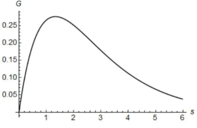
Although the changes mentioned before improve Goodwin’s model by making it more realistic, the weight function chosen doesn’t incorporate the phenomenon of rising wages during a recession. Instead, it slows the growth of wages when employment levels start decreasing. To get a model closer to reality, one should choose a weight function of the form
G(s) =a2se−as, a >0.
This choice of function introduces a delay on how wages react to employment, and assumes a maximum ats= 1
a such thatG(
1
a) = a
e. For the particular case wherea= 0.75the weight function is illustrated in
figure 5.2.
According to Vadasz, choosing this type of weight function would transform the system in (5.11) in
˙
x=η1(1−x)x−θ1xy
˙
y=−η2y+θ2yz1
˙
z1=a(z2−z1) ˙
z2=a(x−z2).
(5.13)
Looking at this model, one can see that the real wages in the second equation will be set according to past employment with dynamic relationship described by last two equations of the system.
Figure 5.2: Weight FunctionG(s) =a2se−as, a= 0.75.
5.2
Palomba’s Model
The author famous for introducing the Lotka-Volterra dynamics in economics is Goodwin (1967). Yet, as pointed out by Massimo di Mateo (1988) [26], the economist Giuseppe Palomba had used these equa-tions in a book published in 1939. Throughout this section we will study Palomba’s work and results concerning the application of Lotka-Volterra dynamics in economics.
Palomba (1939) [12] considers an economy where there are only two types of goods: consumption goods, such as clothing and food, and capital goods, such as buildings and machinery. The model is built under the following assumptions:
Assumption 1: There are two types of goods: goods of typea, which consist of goods ready for im-mediate consumption and goods that directly enter into their production; goods of typeb, namely capital goods that directly enter into the production of other capital goods and only indirectly into the production of consumption goods.
There-fore, some of the commodities of typeaare allocated to categoryb.
Assumption 3: In any given time goods of typeahave a coefficient of increase equal to ǫ1, and this growth may be caused by long-term forces such as productivity and labor force growth. On the other hand, goods of typebhave a coefficient of increase equal to−ǫ2. Sinceǫ1andǫ2are positive constants, these coefficients imply that if there is no change in destination as mentioned in assumption 2, then goods of typeawould increase continuously while goods of typebwould decrease towards zero.
Assumption 4: The coefficient of decrease of goods of typea, due to changes in destination, is equal to−γ1, while the coefficient of increase of the goods of typeb, due to the same reason, is equal toγ2. Here,γ1andγ2are positive constants.
Palomba denoted asC1the volume of the goods of typea, and asC2the volume of the goods of typeb. The assumptions previously made translate into the following equations:
dC1
dt =C1(ǫ1−γ1C2) dC2
dt =−C2(ǫ2−γ2C1)
(5.14)
For the simplicity of of future computations we defineα1 =ǫ1,α2 =−ǫ2,β1 =−γ1andβ2 =γ2. With this notation we obtain a system equivalent to the previous one
dC1
dt =C1(α1+β1C2) dC2
dt =C2(α2+β2C1)
(5.15)
Manipulating system (4.14) we find that
β2dC1 dt −β1
dC2
dt =β2C1α1−α2γ1C1 α2 1
C1 dC1
dt −α1
1
C2 dC2
dt =β1C2α2−α1β2C1.
(5.16)
and if we sum these conditions we get
β2dC1 dt +α2
1
C1 dC1
dt −β1 dC2
dt −α1
1
C2 dC2
dt = 0. Integrating both sides of this equality we obtain
β2C1+α2logC1−β1C2−α1logC2=k′,
wherek′is a constant. Therefore, applying the exponential function to both sides of the equation we get
eβ2C1
Cα2
1 =keβ
1C2
Cα1
wherek=ek′. If we go back to the original notation, the previous equality writes
eγ2C1
C−ǫ2
1 =ke−γ
1C2
Cǫ1
2 . (5.17)
Furthermore, if we let
Y =eγ2C1
C−ǫ2
1 X =e−γ1C2Cǫ1
2
(5.18)
we finally obtain
Y =kX. (5.19)
Palomba studied the behavior of this system following closely the work of Lotka and Volterra on their predator-prey model, where one species feeds on the other. He then made two important observations.
First, he states that the economy’s ondulatory behavior depends solely on the variables involved and their interaction. In other words, he says that cycles are endogenous, self-sustained and consequently non-linear. Considering the year when this study was published this was a surprising statement for the scientific community, since in that period the models proposed by mathematical economists for business cycles were linear and required exogenous factors, such as random shocks, to keep their cyclic behavior. Only in the 1950’s did Goodwin start to develop non-linear models for economic cycles, which lead him to the construction of his famous model for wages and employment presented in the previous section.
Second, he points out that the parametersǫ1,ǫ2,γ1andγ2should be considered general functions of time, instead of static values. With this new feature, Palomba’s model would write
dC1
dt =C1[ǫ1(t) +γ1(t)C1] dC2
dt =C2[ǫ2(t) +γ2(t)C1]
(5.20)
Chapter 6
Conclusions
In nature, species compete, expand and seek resources to continue their existence. The Lotka-Volterra equations model these loss-win interactions and can be used in many fields of study besides the equi-librium of ecosystems. Throughout our work, we have studied some of their possible applications to the banking system and economics.
Studying the application of Lotka-Volterra equations to the banking system, we first looked at three pos-sible models that can describe the relationship between deposit and loan volume on a bank’s balance sheet. The stability of these systems has been analyzed and in the three cases the trivial equilibrium behaves like a saddle point, while the non-trivial equilibria are unstable in the simple model, and condi-tionally stable in the model with Michaelis-Menten response and in the model with reserve requirement. Also, the relationship between mother banks, subsidiary banks and the individuals or companies that use their services has been compared to a three level ecologic food chain. Studying the equilibrium of this dynamical system we found that, under a specific set of conditions involving the parameters of the equations, it is possible to find a stable equilibrium for the system.
Bibliography
[1] V. Volterra. Variazioni e fluttuazioni del numero di individui in specie animali conviventi. Lincei. Mem., pages 31–113, 1926.
[2] V. Volterra. Lec¸ons sur la th ´eorie math ´ematique de la lutte pour la vie. Gauthiers Villar, 1931.
[3] A. J. Lotka. Elements of mathematical biology. Dover Publications, 1925.
[4] S. Chen and S. Bao. A game theory based on predation behavior model.International Conference
on Game Theory, 2010.
[5] M. A. Petersen and I. Schoeman. Modeling of banking profit via assets and return-on-equity.WCE, 2:2–4, 2008.
[6] J. Mukuddem-Petersen, M. A. Petersen, I. M. Schoeman, and B. A. Tau. Dynamic modelling of bank profits. Applied Financial Economics Letters, pages 157–161, 2008.
[7] C. A. Comes. Banking system: Three level Lotka-Volterra model.Procedia Economics and Finance, 3:251–255, 2012.
[8] N. C. Apreutesei. An optimal control problem for Lotka-Volterra system with diffusion. Bul. Inst.
Polytechnic, pages 31–41, 1998.
[9] N. C. Apreutesei. Necessary optimality conditions for a Lotka-Volterra three species system.
Math-ematical Modelling of Natural Phenomena, pages 123–125, 2006.
[10] N. Sumarti and I. Gunadi. Reserve requirement analysis using a dymacial system of a bank based on Monti-Klein model of bank’s profit function.Computers and Mathematics with Application, 2013.
[11] N. Sumarti, R. Nurfitriyana, and W. Nurwenda. A dynamical system of deposit and loan volumes based on the Lotka-Volterra model. AIP Conference Proceedings, pages 92–94, 2014.
[12] G. Palomba. Introduzione allo studio della dinamica economica. Napoli Jovene, 1939.
[13] R. M. Goodwin. A growth cycle. Cambridge University Press, pages 54–58, 1965.
[15] E. Wolfstetter. Fiscal policy and the classical growth cycle. Journal of Economics, pages 93–375, 1982.
[16] M. C. Sportelli. A Kolmogoroff generalized predator-prey model of Goodwin’s growth cycle.Journal
of Economics, pages 35–64, 1995.
[17] K. V. Velupillai. Linear and nonlinear dynamics in economics: The contributions of R. Goodwin.
Economic Notes, pages 73–91, 1982.
[18] P. Flaschel. Some stability properties of Goodwin’s growth cycle. Journal of Economics, pages 63–69, 1984.
[19] D. E. Atkinson. Regulation of enzyme function. Annu. Rev. Microbiol., pages 47–68, 1969.
[20] D. Harvie. Testing Goodwin: growth cycles in ten OECD countries. Cambridge Journal of
Eco-nomics, pages 349–376, 2000.
[21] L. Apedaille, H. Freedman, S. Schilizzi, and M. Solomonovich. Equilibria and dynamics in an economic predator-prey model in agriculture. Mathl Comput Modelling, 19:1–15, 1994.
[22] K. Chakraborty, M. Chakraborty, and T. Kar. Bifurcation and control of a bioeconomic model of a prey-predator system with a time delay. Nonlinear Analysis: Hybrid Systems, pages 613–625, 2011.
[23] C. Michalakelis, C. Christodoulos, D. Varoutas, and T. Sphicopoulos. Dynamic estimation of markets exhibiting a prey-predator behaviour.Expert Systems with Applications, 2012.
[24] S. Baigent. Lotka-Volterra dynamics: an introduction. Preprint, 2010.
[25] T. K. Kar. Stablilty analysis of a prey-predator model incorporating a prey refuge. Communications
in Nonlinear Science and Numerical Simulation, pages 681–691, 2005.
[26] M. di Matteo. Goodwin and the evolution of a capitalistic economy: An afterthought. Berlin Heidel-berg, 1988.
[27] G. Thompson. Sources of financial sociability: Networks, ecological systems or diligent risk pre-parednes? CRESC Working Paper Series, pages 1–17, 2011.
[28] A. Haimovici. A control problem for a Volterra three species system.Mathematica-Revue d’Analyse
Num ´erique et de Th ´eorie de l’Approx., pages 35–41, 1980.
[29] K. Marx. A contribution to the critique of political economy. Progress Publishers, 1859.
[30] J. M. Cushing. Periodic time-dependent predator-prey systems. SIAM Journal of Applied
Mathe-matics, pages 82–95, 1977.
[32] V. Vadasz. Economic motion: An economic application of the Lotka-Volterra predator-prey model. 2007.
[33] E. Chauvet, J. Paullet, J. Previte, and Z. Walls. A Lotka-Volterra three-species food chain.
Mathe-matics Magazine, 2002.
[34] L. Michaelis and M. L. Menten. Die kinetik der invertinwirkung. Biochem, pages 333–369, 1913.
[35] G. Gandolfo. The Lotka-Volterra equations in economics: an italian precursor. Accademia dei
Lincei, pages 347–357, 2017.