Submitted28 November 2015
Accepted 4 March 2016
Published29 March 2016
Corresponding author
Reed A. Cartwright, [email protected]
Academic editor
Jeffrey Ross-Ibarra
Additional Information and Declarations can be found on page 20
DOI10.7717/peerj.1848 Copyright
2016 Furstenau and Cartwright
Distributed under
Creative Commons CC-BY 4.0 OPEN ACCESS
The effect of the dispersal kernel on
isolation-by-distance in a continuous
population
Tara N. Furstenau and Reed A. Cartwright
School of Life Sciences and the Biodesign Institute, Arizona State University, Tempe, AZ, United States of America
ABSTRACT
Under models of isolation-by-distance, population structure is determined by the probability of identity-by-descent between pairs of genes according to the geographic distance between them. Well established analytical results indicate that the relationship between geographical and genetic distance depends mostly on the neighborhood size of the population which represents a standardized measure of gene flow. To test this pre-diction, we model local dispersal of haploid individuals on a two-dimensional landscape using seven dispersal kernels: Rayleigh, exponential, half-normal, triangular, gamma, Lomax and Pareto. When neighborhood size is held constant, the distributions produce similar patterns of isolation-by-distance, confirming predictions. Considering this, we propose that the triangular distribution is the appropriate null distribution for isolation-by-distance studies. Under the triangular distribution, dispersal is uniform over the neighborhood area which suggests that the common description of neighborhood size as a measure of an effective, local panmictic population is valid for popular families of dispersal distributions. We further show how to draw random variables from the triangular distribution efficiently and argue that it should be utilized in other studies in which computational efficiency is important.
SubjectsComputational Biology, Evolutionary Studies, Genetics, Mathematical Biology
Keywords Identity-by-descent, Neighborhood size, Kinship coefficients, Triangular distribution, Simulation, Individual based, Fine scale, Correlograms
INTRODUCTION
A dispersal kernel describes the distribution of Euclidean distances between birth site and reproduction site. Ideally, when modeling dispersal, the dispersal distribution would be selected based on how well it fits the dispersal kernel estimated from natural populations. Classically, dispersal has been modeled as a diffusion process with Gaussian displacement; however, the observed dispersal kernels in many species tend to be more leptokurtic with a higher probability of short and long distance dispersal (Bateman, 1950). In plants, the shape of the dispersal kernel near the origin depends on the mechanism of dispersal; for example, there may be a high peak near the origin for gravity or animal dispersal whereas there may be a minimum near the origin for wind dispersal (Barluenga et al., 2011;Clark et al., 2005).
The shape of the dispersal kernel impacts many population processes including the rate of population expansion (Clark, Lewis & Horvath, 2001;Kot, Lewis & Van den Driessche, 1996), responses to environmental changes (Nathan et al., 2011), local adaptation (Berdahl et al., 2015), speciation (Hoelzer et al., 2008), and the spatial distribution of genetic diversity (Bialozyt, Ziegenhagen & Petit, 2006;Ibrahim, Nichols & Hewitt, 1996). Fat-tailed dispersal kernels, with a higher probability of long-distance dispersal, are a good fit to many empirical data sets (Bullock & Clarke, 2000;Clark et al., 2005;Gonzàlez-Martìnez et al., 2006;Martìnez & Gonzàlez-Taboada, 2009;Klein et al., 2006). Many studies have shown that population models behave differently when fat-tailed dispersal distributions are used instead of Gaussian dispersal.Kot, Lewis & Van den Driessche (1996)demonstrated that population spread is sensitive to the shape of the dispersal kernel and models using a normal distribution underestimated the rate of invasion compared to fat-tailed distributions. Nathan et al. (2011)found that long distance dispersal plays a large role during range shifts of wind-dispersed trees in response to projected climate changes.Houtan et al. (2007) showed that heavy tailed dispersal kernels were a better fit for dispersal of Amazonian birds but the shape of the dispersal kernel can change in response to forest fragmentation.
While the shape of the dispersal kernel impacts many population processes at different scales, it remains unclear how it effects patterns of isolation-by-distance within a continuous population. It has been argued that the number of long-distance dispersal events will not have a noticeable effect because new long-distance alleles are more likely to be lost due to drift than become established at the new location (Epperson, 2007;Ibrahim, Nichols & Hewitt, 1996). On the other hand, the shape of the dispersal kernel near the origin may have a significant impact on the overall rate of migration. In plants, this could result in a higher probability of self-fertilization and/or a reduction in the number of successful offspring when there is density dependent regulation (Barluenga et al., 2011;Howe, Schupp & Westley, 1985;Moyle, 2006).
density (Malécot, 1969; Maruyama, 1970; Sawyer, 1977) but these results hold when considering continuously distributed populations with spatial clustering (Barton et al., 2013). In two dimensions, the relationship between the probability of identity-by-descent and the log of distance is linear over a certain range of distances and the relationship is proportional to 1/(Deσ2) whereDeis the effective population density and 2σ2is the mean
squared distance of dispersal (i.e., non-central second moment of Euclidean distance;
Barton et al., 2013;Malécot, 1969;Rousset, 1997;Rousset, 2004;Wright, 1946). Over this range, the slope of the probability of identity-by-descent function is independent of most aspects of the dispersal distribution except for 2σ2; however, when the distance between individuals falls below the range, the shape of the dispersal distribution becomes important (Rousset, 1997). This suggests that as long as 2σ2stays constant, any dispersal distribution will produce similar patterns of isolation-by-distance. However, Rousset argues that the magnitude of genetic differentiation will always depend on the shape of the distribution (Rousset, 1997;Rousset, 2008).
Despite the increase in the use of spatially explicit simulations in studies of spatial genetic structure, it remains unclear whether the shape of the dispersal kernel should be considered. There has not been a clear comparison of how the shape of different dispersal kernels affect observable patterns of isolation-by-distance in these simulations. Here we attempt to offer such a comparison using a spatially-explicit, individual-based model to simulate local dispersal in a continuous population to determine if patterns of isolation-by-distance vary based on the shape of several different dispersal distributions: Rayleigh, half-normal, exponential, triangular, gamma, Lomax, and Pareto. Each dispersal distribution has a different shape, but they can be parameterized such that their non-central second moment is 2σ2. If the simulations reveal a similar pattern of isolation-by-distance across all dispersal distributions, we can conclude that, for a wide range of dispersal distributions, 2σ2is the main determining factor of how genetic similarity declines with increasing distance in a continuous population. Consequently, when designing isolation-by-distance simulations, researchers may choose a dispersal distribution based on computational needs instead of biological fit.
Wright (1946)uses the term ‘‘neighborhood’’ to describe a local population from which parents are randomly drawn. He measures the magnitude of the effective size of the neighborhood,Nb, as the inverse of the probability that two gametes at the same location
came from the same parent. Assuming dispersal is normally distributed along each axis, he calculated thatNb=4π σ2De, whereDe is the effective density of individuals, and 2σ2
is the mean squared distance of dispersal. In his model this captures 86.5% of parents of central individuals. Although Wright assumed Gaussian dispersal, his formula can be used to calculateNbfor many different dispersal models at equilibrium due to the central-limit
theorem.Nbis important because it helps define the rate of decay of genetic similarity over
spatial distance, i.e., the amount of isolation-by-distance in a population (Barton et al., 2013;Rousset, 1997;Rousset, 2000).
triangular distribution:f(r;σ)=r/(2σ2), where 2σ2 is again the non-central second moment. This type of neighborhood is similar to the neighborhood defined in the spatially continuous 3-Fleming-Voit disc model in which a number of parents,v, are chosen uniformly at random from a disc with radius r to replace a fractionuof the population (Barton et al., 2013). In this model, neighborhood size is defined by the ratio
v/uand the individuals occupying the disc constitute a panmictic population. If 100% of the population is replaced (u=1), the definition of neighborhood size reduces to the number of individuals competing for the central location.
Below, we demonstrate that patterns of isolation-by-distance are equivalent for different dispersal kernels with the same second moment, and discuss the use of the triangular distribution to model dispersal in a continuous population.
METHODS
Simulation
In our individual-based simulation, a population exists on a 100×100 rectangular lattice (cf.Epperson, 1995;Epperson & Li, 1997;Epperson, 2007;Hardy & Vekemans, 1999). Individuals are uniformly spaced with a single individual per cell. Each individual contains one haploid locus. The initial population of 10,000 individuals each carry a unique allele. Generations are discrete, and individuals reproduce by generating 15 clonal offspring that experience mutations according to the infinite alleles model at rate µ. All starting and mutant alleles are selectively neutral.
The offspring disperse from the parent cell following a given dispersal distribution. The landscape boundaries are absorbing, and when offspring disperse off of the lattice they are lost. Offspring that land in the same cell will compete to become a parent in the next generation. Because all alleles are selectively neutral, a single successful offspring is uniformly selected for each cell. To avoid storing all the offspring in memory until dispersal is completed, we use a reservoir sampling method to immediately accept or reject offspring when they land on a cell (Vitter, 1985). This method allows us to keep track of two randomly chosen offspring per cell. The first offspring becomes a parent in the next generation and the second individual is recorded to measure the probability of identity-by-descent for offspring competing for the same cell. While it is possible for a cell to remain empty after dispersal, we determined that when each parent generates 15 offspring the number of empty cells per generation is negligible so we assume a constant homogeneous population density.
Modeling Dispersal
Once the angle and distance are drawn, the final position is determined by converting the polar coordinates into rectangular coordinates and adding them to the parent’s position. The new coordinates are then rounded to determine the integer coordinates of the destination cell. This dispersal scheme is similar to the centroid-to-area approximation of continuous dispersal kernels described by Chipperfield et al. (2011), which showed minimal deviation from expectations especially when cell length is less than the expected distance.
We looked at seven different dispersal distance kernels (Fig. S1): Rayleigh, exponential, half-normal, triangular, gamma, Pareto, and Lomax. We chose these distributions because they provide a range of shapes for short, intermediate, and long distance dispersal.
The Rayleigh is a distribution of Euclidean distances that result from bivariate normal displacement along thexandy axis. The Rayleigh distribution follows the assumptions ofWright (1946)’s two-dimensional isolation-by-distance model.
The exponential distribution is more leptokurtic with higher probability of dispersal at short and long distances and less at intermediate distances. The exponential tail is the boundary that separates truly heavy-tailed distributions with potentially infinite higher moments from distributions with all moments finite. The distinction is important because leptokurtic, heavy-tailed dispersal kernels are typically a better fit to observed dispersal in nature (Clark, 1998).
The half-normal distribution is equivalent to a normal distribution that has been folded over they-axis. In this case, Euclidean distance is simply the absolute value of normally distributed random variables. The half-normal is a monotonically decreasing distribution with a convex shoulder near zero. This distribution has a higher probability of dispersal at intermediate distances compared to the exponential.
The triangular distribution is typically defined using three points: a lower limit,a, an upper limit,b, and a mode,c. Here we use a special case of the triangular distribution where
a=0 andb=c=2σ. We chose this special case of the triangular distribution because in our dispersal function it will return polar coordinates that are uniformly sampled from within a circle with area 4π σ2which is the same as the neighborhood area (see proof in
Appendix A). The triangular distribution is also the only one of our distributions that has a finite range,r∈ [0,2σ].
Unlike the previous single parameter distributions, the final three distributions have an additionalα shape parameter. The gamma distribution is equivalent to the exponential distribution whenα=1, and asα increases the distribution becomes more symmetrical with a higher probability for intermediate distances and a lower probability for short distances.
The Lomax and Pareto distributions are both heavy-tailed power-law distributions. Then-th moments are finite only whenα >n. The support for the Pareto distribution,
r∈ [xmin,+∞), begins at a parameter xmin>0. The Lomax distribution is a Pareto distribution that has been shifted so that the support begins at zero. We chose values ofα
The dispersal function is executed over 100-billion times per simulation, and thus it is important to make the implementation as efficient as possible. With this aim, we used an xorshift algorithm for uniform pseudo-random number generation and the ziggurat rejection sampling algorithm when applicable (Marsaglia & Tsang, 2000b;Marsaglia, 2003). We used two different versions of the ziggurat algorithm to draw distances from the exponential and half-normal distribution. For the gamma distribution we used a rejection sampling method that uses the ziggurat algorithm to draw normal variates (Marsaglia & Tsang, 2000a). Random variables from the Pareto distribution are generated byxmineX/a whereX is an exponentially distributed random variable that we draw using the ziggurat algorithm. The Lomax distribution is sampled similarly:xmineX/a−xmin.
In addition to generating random distances, the dispersal function requires costly conversions from polar to Cartesian coordinates. We were able to avoid this conversion for the Rayleigh and triangular distributions. We simulated the Rayleigh distribution by drawing vertical and horizontal offsets from independent normal distributions using the ziggurat algorithm. For the triangular distribution, we developed a discrete sampling algorithm using the alias method that allows us to draw the vertical and horizontal offsets simultaneously in constant time (Vose, 1991). SeeAppendix D for a description of the algorithm, andAppendix Efor an analysis of its superior efficiency compared to the other distributions we used.
Analysis
A simulation was run for each of the seven types of dispersal distributions under 4 levels of dispersal (σ=1, 1.5, 2 and 4) with a mutation rate ofµ=10−4. Each simulation was run for a burn-in period of 10,000 generations to allow the population to reach a mutation-drift equilibrium. After the burn-in, data was collected from populations that were 1,000 generations apart to decrease the correlation between them for a total of 2,000 replicate populations per simulation. In each population, a straight transect of 50 individuals was sampled from the center of the landscape to avoid measuring edge effects.
From the transect, all possible pairs of individuals were placed into distance classes based on the geographical distance between the pair. The number of pairs that shared an identical allele was determined and recorded as a proportion of the total number of pairs in the distance class. The probabilities for each distance class were then averaged over all sampled populations. Under this sampling scheme, the number of pairs per distance class decreases as distance increases so in distance class 50 there is only one pair sampled per population.
The parameters for each dispersal distribution were calculated so that E[X2] =2σ2; the calculations are reflected in the probability distribution functions inFig. S1. Due to the discrete nature of the lattice, some parameters values were adjusted slightly until the simulations produced an average, observed, squared distance between parent and offspring,
s2, that was within 5% of the expected value,σ2. Three of the distributions require a second
Under isolation-by-distance, individuals geographically near one another will tend to be genetically similar, and this similarity will decrease as the distance between pairs of individuals increases. Therefore, isolation-by-distance is described by constructing correlograms of genetic similarity between individuals versus the distance between them. Genetic similarity can be measured using identity-by-descent, identity-by-state, relatedness, conditional kinship, or F-coefficients and can be based on coalescent times, an ancestral population, or the current population (Hardy & Vekemans, 1999;Hardy, 2003;Malécot, 1969;Rousset, 1997;Rousset, 2002;Wang, 2014). For two-dimensional populations, genetic similarity is often plotted against the log-distance separating pairs because theory predicts that this relationship is approximately linear (Barton et al., 2013;Hardy & Vekemans, 1999;
Rousset, 2000).
We recorded the probability of identity-by-descent for pairs of individuals in each distance class. Under the infinite alleles model, pairs of individuals were considered identical-by-descent if they shared the same allele. The probability of identity-by-descent in each distance class depends on the mutation rate; the probability will be greater when there are fewer alleles. For more consistent results that are nearly independent of mutation rate, the probability of identity is often calculated as a ratio that measures genetic similarity (or differentiation) relative to a particular reference group. We calculated the kinship coefficient which measures the correlation of genetic similarity between pairs of individuals a certain distance apart relative to the genetic similarity in the whole sample.
Fr=
pij−¯p
1−¯p ≈
E[T] −Eij[T]
E[T] . (1)
Here pij is the probability of identity-by-descent between haploid individualsi and
j at distancer and ¯pis the probability of identity-by-descent between random haploid individuals in the current sample (Hardy & Vekemans, 1999). The kinship coefficient is related to differences in the expected coalescent times, T, between a specific pair of individuals and a random pair in the population (Barton et al., 2013). Kinship coefficients were calculated for each transect and then averaged across transects for each distance class. Since this statistic is highly dependent on the sampling scheme, we sampled the same transect in all simulations.
We also calculated thear parameter ofRousset (2000):
ar=
p0−pij
1−p0
(2)
which measures genetic differentiation over distance relative to the probability of identity-by-descent within a location. Thear parameter is independent of sampling scheme, but
it does depend on the level of local identity-by-descent,p0, in the population such that
For each simulation, we calculated the average number of unique alleles in a 50-individual transect (¯k) and the average squared distance between parents and offspring (2s2). Using
¯k, we estimated the population-level diversity,θˆk (Ewens, 2004eq. 9.32) and estimated
effective haploid population size asNˆe=θˆk/2µand effective density asDˆe=Nˆe/A, where
A=10,000.
Finally, we estimated neighborhood size using two different methods. First we used our estimated demographic parameters to calculate neighborhood size as the product
ˆ
Nb=4πs2Dˆe. We calculated an estimate from samples from each population and calculated
an average over all populations. We then estimated neighborhood size using the regressions of bothFr andar on the log of distance. The slope of thear regression is an estimate of
1/2π σ2Deand the slope ofFrregression is an estimate of−(1−F0)/2π σ2De(Barton et al., 2013;Hardy & Vekemans, 1999;Rousset, 2000). We performed the regression for distance classes between 5 and 35. We estimated the slope from each population sample then pooled the data from all the samples to get a combined slope estimate.
RESULTS
Behavior of dispersal distributions
The more leptokurtic distributions (exponential, gamma-1 and Lomax) with a high probability peak near zero have a much higher probability of not dispersing from the original cell, especially whenσ is low. The Pareto distribution, which has a fat tail but has been shifted so it does not have a peak at zero, has a very low probability of not dispersing. Under the gamma distribution as theα parameter increases, the probability of remaining at the origin decreases; whenα=8 the probability is nearly zero for all values ofσ.Figure S2shows the empirical cumulative distributions generated from 10,000 simulated dispersal events from each distribution. The probability of not dispersing from the original cell is indicated by the height of the left-most horizontal line for each distribution.
The average squared parent–offspring dispersal distance, s2, observed for each distribution was very similar with a relative error of less than 5% from the expected
σ2 value (Table 1); however, the distribution of these values over sampled generations varied (Fig. S3A). Expectedly, the thin tailed or no-tail (triangular) dispersal distributions have the smallest variance because their properties are easier to represent with a small number of samples. The Lomax distribution has the highest variance with the median falling slightly below the expected value.
Figure S3Bshows the distribution of the average cubed parent–offspring dispersal distances, s3, for each transect. The theoretical third moment of the Lomax and Pareto distributions is infinite, while it is not possible to simulate this on a finite landscape, we do observe values ofs3that are several orders of magnitude larger than distributions with finite third moments. The distribution ofs2ands3for the Lomax and Pareto distributions both have a large positive skew.
Allelic diversity
Table 1 Estimated neighborhood sizes are similar across all dispersal distributions.Estimates of allele diversity,θˆk, effective population density,Dˆe, dispersal,s2, and neighborhood size. Neighborhood size is
estimated two different ways.Nˆb(θ)is 4πs2Dˆ
ewhereDˆeis estimated fromθˆk.Nˆb(ar)is twice the inverse of the slope ofarand the log of distance. The expected neighborhood size (4π σ2·1) is 12.56, 28.28, 50.26,
and 201.06 forσ=1, 1.5, 2, and 4, respectively.
σ
ˆ
θk Deˆ s2 Nbˆ (θk) ˆ Nb(ar)
ˆ
θk Deˆ s2 Nbˆ (θk) ˆ Nb(ar)
1 1.5
Ray 1.82 0.91 0.99 11.31 13.07 1.83 0.91 2.33 26.79 31.16 Exp 2.09 1.04 1.04 13.70 14.32 2.04 1.02 2.26 29.04 29.00 Nor 1.94 0.97 0.98 11.94 13.49 1.91 0.95 2.31 27.69 30.61 Tri 1.82 0.91 1.00 11.37 13.58 1.83 0.92 2.36 27.18 31.02 Gam 1 2.07 1.04 1.05 13.63 14.41 2.01 1.00 2.32 29.22 30.07 Gam 2 1.89 0.94 0.98 11.62 12.80 1.85 0.92 2.32 26.98 30.13 Gam 4 1.83 0.92 1.00 11.49 12.88 1.87 0.94 2.32 27.31 28.27 Gam 8 1.80 0.90 1.01 11.45 13.31 1.79 0.90 2.32 26.16 29.91 Lom 2.4 2.97 1.49 1.06 19.70 13.41 2.62 1.31 2.16 35.53 26.65 Lom 2.6 2.88 1.44 0.97 17.61 13.23 2.47 1.24 2.34 36.25 26.11 Lom 2.8 2.73 1.36 1.04 17.78 12.82 2.41 1.21 2.22 33.66 25.30 Lom 3 2.72 1.36 1.00 17.07 14.28 2.36 1.18 2.34 34.71 28.50 Par 2.4 1.98 0.99 0.98 12.18 11.71 1.93 0.97 2.19 26.56 27.12 Par 2.6 1.95 0.98 1.04 12.74 13.82 1.81 0.91 2.28 25.98 27.95 Par 2.8 1.90 0.95 0.97 11.57 12.25 1.85 0.93 2.25 26.16 30.85 Par 3 1.89 0.95 0.99 11.80 13.56 1.89 0.94 2.24 26.54 29.79
2 4
(Fig. S4). The expected number of alleles under the infinite alleles model is equal to
Pn−1
i=0θ /(θ+i)=7.03 wheren=50 is the number of individuals in the sampled transect. The Lomax distributions have a higher median number of alleles at lower values ofσ but this gets closer to the expected value whenσ >2. The average diversity is also slightly elevated for the exponential and gamma-1 simulations.
Differences in effective population size between simulations can be measured by comparing the number of unique alleles observed in the transects. Different dispersal kernels produce similar levels of diversity, except for the Lomax distributions which have a higherθk and consequently a larger effective population size (Table 1).
Spatial autocorrelation and isolation-by-distance
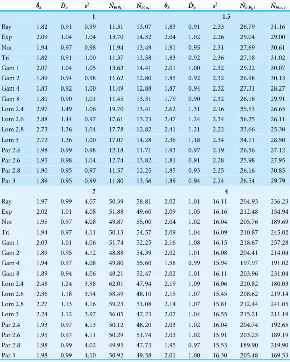
To describe the patterns of isolation-by-distance, we first measured the average probability of identity-by-descent for each sampled population as a function of distance. All dispersal kernels produced very similar patterns of isolation-by-distance especially for larger distance classes (Fig. 1). The probability of identity-by-descent is higher at small distance whenσ
is small but the relationship flattens out whenσ=4. Differences between the different dispersal distributions become apparent when the distance between individuals is small. The more leptokurtic dispersal distributions have a steeper incline as distance decreases and they have a higher probability of autozygosity at distance class zero. The plots for the triangular distribution nearly perfectly overlap the plots for the Rayleigh distribution in all cases.
Because the probability of identity-by-descent is sensitive to differences in the number of alleles present in the sample, we also calculated the pairwise-kinship coefficient over the log of distance (Fig. 2). The kinship coefficient shows how much more or less similar pairs of individuals in a given distance class are compared to the sample as a whole. The kinship coefficient is nearly independent of differences in allele number and there is much better overlap of the plots for the different dispersal distributions. When the kinship coefficient is plotted against the log of distance there is a negative linear relationship over a certain range of distances (Hardy & Vekemans, 1999). The slope of this linear range is also similar across distributions for each value ofσ.
Finally, we plotRousset (2000)’sar parameter against the log of distance. There is a
positive linear relationship betweenar and the log of distance (Fig. 3). The slope ofar is
fairly similar among the dispersal distributions for a given value ofσ. However, there is less overlap in the plots for the different dispersal distributions because the overall amount of differentiation varies.
Estimated neighborhood size
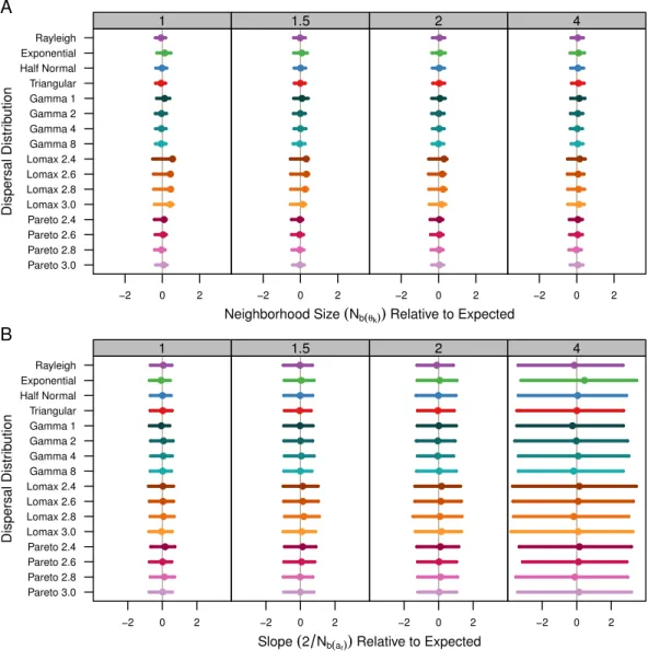
TheNˆb(θk)estimates are shown inTable 1andFig. 4A.Table 1shows the average estimate
over all population samples. The colored dots inFig. 4Ashow this same average relative to the expected values and the bars represent the middle 50% of the individual sample estimates. As mentioned previously, the populations with Lomax dispersal tend to have a greater number of unique alleles and this translates to higherθˆk, higher effective population
Figure 1 Identity-by-descent is similar between different dispersal models.Each plot shows the average probability of identity-by-descent for pairs of individuals in each distance class. Each panel represents sim-ulations run with differentσparameters (gray box) for different groups of dispersal distributions.
skewed towards lower values. As a result, the estimates ofNˆb(θk)for the Lomax distribution
appear to be higher on average but the estimates are skewed. Otherwise, the estimates for the other dispersal distributions are similar and close to the expected values.
Table 1shows theNˆb(ar)estimates calculated as the twice the inverse of the regression of
ar and the log of distance for the pooled sample data. Estimates using the slope of theFr
Figure 2 Kinship coefficients are similar between different dispersal models.Each plot shows the aver-age kinship coefficient for pairs of individuals over the log of the distance between them. Each panel rep-resents simulations run with differentσparameters (gray box) for different groups of dispersal distribu-tions. The gray dashed line is at zero so values above the line are more similar than the sample as a whole while values below the line are less similar than the population as a whole.
DISCUSSION
Figure 3 Slopes of genetic differentiation are similar between different dispersal models.Each plot shows the average differentiation,ar, for pairs of individuals over the log of the distance between them.
Each panel represents simulations run with differentσparameters (gray box) for different groups of dis-persal distributions.
events do not leave the parent cell. The Pareto and Lomax distributions share a similar shape and a wide tail, but unlike the Lomax distribution, the mode of the Pareto is greater than zero and almost all dispersal events leave the original cell. We refer back to the differences between the Lomax and the Pareto when we discuss whether we can differentiate results that are specific to dispersal with a high peak at zero or are more general to wide-tailed dispersal.
Figure 4 Estimated neighborhood sizes are similar across all dispersal distributions.Neighborhood size is estimated two different ways. (A)Nb(θk)is 4πs
2Dˆ
ewhereDˆeis estimated fromθˆk. The dot is the
av-erage from all populations samples and the bars represent the middle 50% of estimates from individual samples. (B) The slope estimates, 2
Nb(ar), ofarand the log of distance. The dots represent the slope estimate
from the combined data from all samples and the bars represent the middle 50% of slopes from individual samples.
simulations falls near the expected value, it seems likely that the higher allelic diversity in the Lomax simulations is due to the high probability of not dispersing. This is supported by the fact that the average diversity is slightly higher for the exponential and gamma-1 as well. When dispersal is unlikely to occur outside of the original cell, the number of migrants is low and the pool of offspring before competition will consist mostly of offspring from the same parent. It is unlikely that migrants will become established at their new location after competition and thus more alleles will be maintained.
occupying a finite lattice with absorbing boundaries to better understand the effect of the dispersal kernel on isolation-by-distance models on a more natural landscape. As expected under isolation-by-distance, the probability of identity-by-descent between neutral alleles in pairs of individuals decreases as the distance between them increases. When neighborhood size is small, the relationship is very pronounced with a high initial probability that quickly declines. As neighborhood size increases (σ=4), this relationship nearly disappears. This is similar to two-dimensional stepping stone models that show strong differentiation between populations whenNm≪1 and little differentiation when
Nm>4 (Kimura & Maruyama, 1971).
Simulations with our different dispersal kernels show a strikingly similar pattern of isolation-by-distance. However, theory predicts that when distance is small, deviation in the shape of the dispersal kernel relative to the Rayleigh distribution will become important (Rousset, 1997;Rousset, 2000). This is evident in our results when we compare the probabilities of identity-by-descent at small distances between the different dispersal kernels. When the dispersal kernel is leptokurtic, the probability is higher between individuals occupying the same location and it is slightly lower for short distances compared to the Rayleigh results. The pattern of identity-by-descent in other distributions, including the triangular are nearly identical to the Rayleigh. The situation is similar for the pairwise kinship except there is even greater similarity between the different dispersal kernels.
Rousset (2008)makes it clear that the increase of genetic differentiation with distance is robust to the shape of the dispersal kernel but the overall magnitude of differentiation will depend on the shape of the kernel. Looking at the relationship betweenar and the log
of distance for our simulations, we can see that the slope for each distribution is similar for larger distance values but the plots are shifted up or down depending on kurtosis. Compared to the other wide tailed distributions, the Pareto distribution is not shifted upward due to the lack of dispersal at the origin. Thear statistic is a ratio that compares the
amount genetic differentiation between individuals at certain distance to the differentiation within a single individual. When the probability of identity-by-descent within an individual is high, the differentiation between neighbors will appear much higher due to a steep initial drop in identity. As a result, thear statistic will be greater for leptokurtic distributions even
if the actual probability of identity is similar to other distributions.
As expected, the neighborhood-size estimates are similar to the expected value for all simulations. Neighborhood size was slightly higher for the Lomax simulations when using allele diversity to estimate effective density. Otherwise, the slopes of the regression methods were similar and thus predicted similar neighborhood sizes. This reconfirms that neighborhood size is a robust descriptor of the decrease of genetic identity with distance. It also seems clear that fat-tailed dispersal kernels do not have much of an effect in isolated continuous populations.
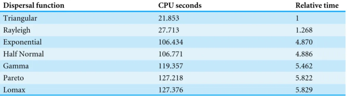
Table 2 Triangular dispersal algorithm is the most efficient.Execution time and relative time for 109 dispersal events from different dispersal functions ordered from most to least efficient.
Dispersal function CPU seconds Relative time
Triangular 21.853 1
Rayleigh 27.713 1.268
Exponential 106.434 4.870
Half Normal 106.771 4.886
Gamma 119.357 5.462
Pareto 127.218 5.822
Lomax 127.376 5.829
The triangular dispersal model can serve as a null model for the probability that two lineages will meet and coalesce in a previous generation. Identity-by-descent may be defined as the total probability of coalescence between the current generation,t0, and a generation at some time t in the past (Rousset, 2002). When a population is not panmictic due to limited dispersal, the time to coalescence depends on the probability that the two lineages will move close enough together so that there is some probability that they shared a parent in the previous generation. When the dispersal kernel has an infinite tail, there is always some small probability that two individuals coalesce even if they are very far apart. Because the triangular distribution is finite with a maximum distance of 2σ, the probability that two individuals coalesce in the previous generation is 1/(4π σ2D) if they are separated by a distance less than 2σ and zero otherwise.
The triangular distribution allows us to simulate dispersal more efficiently than other dispersal kernels because it is uniform over a finite area. It allows us to easily pre-compute probabilities of dispersal to neighboring cells and use an efficient discrete sampling algorithm to sample dispersal positions. A similar approach is possible for other dispersal distributions. For distributions with infinite tails this would require defining a truncated distribution which captures the bulk of the dispersal probabilities. Then, for two dimensions, double integrals would need to be calculated to determine the probabilities of dispersal to locations on the lattice. These pre-computations are laborious because in addition to the double integrals, many cells will have non-zero probabilities. For the triangular distribution, only cells in a radius of 2σwill have non-zero probability and since the distribution is uniform, the probabilities are easy to calculate.
the rate of population expansion, colonization, responses to climate change, population fragmentation and the movement of genes between locally adapted populations. Each of these processes will be affected by the dispersal distribution chosen for the simulation. However, when simulating a population structured by isolation-by-distance, the shape of the dispersal kernel does not appear to have a strong effect in a finite, isolated population. Because speed is an important factor in deploying isolation-by-distance simulations in analytical contexts, e.g., approximate Bayesian computation, we recommend using the triangular distribution when long distance dispersal and other features of the dispersal kernel can safely be ignored.
ACKNOWLEDGEMENTS
The authors would like to thank R Schwartz, D Winter and S Wu for helpful comments, and K Dai for programming tips. The authors would also like to thank Jeffrey Ross-Ibarra, Michael Blum, and one anonymous reviewer for their suggestions which improved this manuscript.
APPENDIX A. TRIANGULAR DISTRIBUTED DISTANCES CAN
PRODUCE A UNIFORM DISTRIBUTION ON A DISK
Proof
The probability density of a uniform distribution over a finite two-dimensional shape is defined as:
f(x,y)=
1
area ofS if (x,y)∈S
0 otherwise
where (x,y) are coordinates on the Cartesian plane andSis the set of all points within the shape. A uniform distribution on the region bounded by a circle is defined by π1R2
whereRis the radius of the circle. We are interested in a circle with radiusR=2σand area
A=4π σ2so the non-zero part of the joint probability distribution is given by:
f(x,y;σ)= 1
4π σ2 whenx 2
+y2≤4σ2.
Using the change of variables theorem for polar coordinates, (r,θ), we have:
ZZ
D
f(x,y) dxdy = ZZ
D∗
f(rcosθ ,rsinθ)r dr dθ
= ZZ
D∗
r
4π σ2 drdθ = ZZ D∗ 1 2π r
2σ2 dr dθ .
We then integrate out the angleθ to isolate the distribution of distance,f(r;σ):
f(r;σ)=
Z 2π
0
r
4π σ2 dθ=
r
4π σ2θ
2π 0 = r
The distribution of distances is equivalent to a special case of the triangular distribution. The probability density function for the triangular distribution is
f(r;a,b,c)=
0 forr<a
2(r−a)
(b−a)(c−a) fora≤r≤c 2(b−r)
(b−a)(b−c) forc≤r≤b 0 forr>b
whereais the lower limit,bis the upper limit, andcis the mode. In the special case, we set
a=0 andb=c=2σ. The probability density function for the special case of the triangular distribution simplifies to
f(r;σ)= ( r
2σ2 for 0≤r≤2σ
0 otherwise
APPENDIX B. XORSHIFT RANDOM NUMBER GENERATOR
Xorshift is a type of pseudo-random number generator that relies on exclusive-or and bitshift operators (Marsaglia, 2003). Xorshift is one of the most efficient, high-quality random-number generators known. Our implementation is a 64-bit xorshift with shift parameters (5, 15, 27) added to a Weyl series to decrease bit correlations (Brent, 2007). It passes the BigCrush tests in the TestU01 suite (L’Ecuyer & Simard, 2007).
APPENDIX C. GENERATING FROM A CONTINUOUS
TRIANGULAR DISTRIBUTION
Inverse sampling can be used to generate values from a triangular distribution. Note that we are only working with monotonically increasing triangular distributions and not more general formulations. If uis uniformly distributed in (0,1), the value d=2s√u
has a triangular distribution with parameter s. However, a modified rejection sampling algorithm is faster. Ifu1andu2are independent and uniformly distributed in (0,1), then
d=2smax(u1,u2) also has a triangular distribution. Because we can generate 32-bit values for bothu1andu2 from a single 64-bit random number, this second algorithm is more efficient than the first. While it is possible to construct a ziggurat algorithm (Marsaglia & Tsang, 2000b) for a triangular distribution, our second algorithm is more efficient because it involves fewer steps and never rejects.
rejection sampler took 1,911 s. The maximum algorithm produced faster execution, but only sped up the tests by 3% over sqrt.
APPENDIX D. GENERATING DISCRETE TWO-DIMENSIONAL
DISPERSAL FROM A TRIANGULAR DISTRIBUTION
We can use the maximum algorithm above to generate the values in polar coordinates and convert them to Cartesian coordinates; however, this requires calculating sine and cosine functions, which we would rather not do. When modeling dispersal on a lattice, the bounded nature of the triangular distribution allows dispersal to be modeled discretely. To discretize this distribution on a rectangular lattice we must determine the probabilities for each cell which are proportional to the area of the cell that is covered by a disk of radius
r=2σ(centered on a focal cell). The algorithm described here produces probability tables by calculating the appropriate area for each cell and dividing by the total area. We assume that cells are squares with unit area.
Since the disk is symmetrical, this algorithm may be simplified by calculating areas for quadrant I of the disk and mirroring those values to the other quadrants. We further simplify by calculating approximately half of the areas for quadrant I and mirroring those as well. Note that this results in cells along thexandyaxes having an area of 1/2. Starting at the center of the focal cell (y0=0), we record the top/bottom boundary of each cell along they-axis up to the radius:y1=0.5, y2=1.5,...,yn=n−0.5 wheren=supn∈Zyn≤r.
Next we calculate the area of the first column of cells which has a left boundary atx0=0 and a right boundary atx1=min(0.5,r):
A=
Z x1
x0 p
r2−x2dx.
Starting with the bottom cell, we check if the area of a cell is less than the area of the column. If so, the cell is completely contained in the disk, and the cell is assigned a weight equal to its area. Its area is then subtracted from the area of the column. We continue this procedure until the the area of last cell is less than the remaining area of the column and assign the final cell a weight equal to the remaining area in the column.
Our implementation of a discretized triangular kernel can be found in src/disk.h and src/disk.cpp in the source code. Code for generating an alias table can be found in src/aliastable.h.
APPENDIX E. RELATIVE EXECUTION TIME OF DISPERSAL
FUNCTIONS
To compare the run time for the different dispersal functions we simulated one dispersal event from each cell on a 100×100 landscape 100,000 times for a total of 109dispersal events. For each simulationσ=1, andα=3 for the two parameter distributions. The CPU time was averaged over 5 different runs (Table 2). Our implementation of the triangular distribution was the most efficient followed by the Rayleigh which took about 26.8% longer on average. The half-normal and the exponential functions had similar execution times but took nearly 5 times longer than the triangular function. The gamma, Pareto, and Lomax were the least efficient functions running over 5 times longer than the triangular function.
ADDITIONAL INFORMATION AND DECLARATIONS
Funding
The authors received funding from the School of Life Sciences, Arizona State University for this work. The funder had no role in study design, data collection and analysis, decision to publish, or preparation of the manuscript.
Grant Disclosures
The following grant information was disclosed by the authors: School of Life Sciences, Arizona State University.
Competing Interests
Reed A. Cartwright is an Academic Editor for PeerJ.
Author Contributions
• Tara N. Furstenau conceived and designed the experiments, performed the experiments, analyzed the data, contributed reagents/materials/analysis tools, wrote the paper, prepared figures and/or tables, reviewed drafts of the paper.
• Reed A. Cartwright conceived and designed the experiments, contributed reagents/ma-terials/analysis tools, wrote the paper, reviewed drafts of the paper.
Data Availability
The following information was supplied regarding data availability:
Source code for simulations can be found athttps://github.com/tfursten/IBD/tree/vpub. Simulation parameters and results can be accessed at10.6084/m9.figshare.1611097.
Supplemental Information
REFERENCES
Barluenga M, Austerlitz F, Elzinga JA, Teixeira S, Goudet J, Bernasconi G. 2011.
Fine-scale spatial genetic structure and gene dispersal inSilene latifolia.Heredity
106:13–24DOI 10.1038/hdy.2010.38.
Barton NH, Etheridge AM, Kelleher J, Véber A. 2013.Inference in two dimensions: Allele frequencies versus lengths of shared sequence blocks.Theoretical Population Biology87:105–119DOI 10.1016/j.tpb.2013.03.001.
Bateman AJ. 1950.Is gene dispersal normal?Heredity 4:353–363
DOI 10.1038/hdy.1950.27.
Berdahl A, Torney CJ, Schertzer E, Levin SA. 2015.On the evolutionary interplay between dispersal and local adaptation in heterogeneous environments.Evolution
69:1390–1405DOI 10.1111/evo.12664.
Bialozyt R, Ziegenhagen B, Petit RJ. 2006.Contrasting effects of long distance seed dispersal on genetic diversity during range expansion.Journal of Evolutionary Biology
19:12–20DOI 10.1111/j.1420-9101.2005.00995.x.
Brent RP. 2007.Some long-period random number generators using shifts and xors.
ANZIAM Journal48:C118–C202.
Bullock JM, Clarke RT. 2000.Long distance seed dispersal by wind: measuring and modelling the tail of the curve.Oecologia124:506–521DOI 10.1007/PL00008876.
Cartwright RA. 2009.Antagonism between local dispersal and self-incompatibility systems in a continuous plant population.Molecular Ecology 18:2327–2336
DOI 10.1111/j.1365-294X.2009.04180.x.
Chesson P, Lee CT. 2005.Families of discrete kernels for modeling dispersal.Theoretical Population Biology67:241–256 DOI 10.1016/j.tpb.2004.12.002.
Chipperfield JD, Holland EP, Dytham C, Thomas CD, Hovestadt T. 2011.On the approximation of continuous dispersal kernels in discrete-space models.Methods in Ecology and Evolution2:668–681DOI 10.1111/j.2041-210X.2011.00117.x.
Clark JS. 1998.Why trees migrate so fast: confronting theory with dispersal biology and the paleorecord.The American Naturalist 152:204–224DOI 10.1086/286162.
Clark JS, Lewis M, Horvath L. 2001.Invasion by extremes: population spread with variation in dispersal and reproduction.The American Naturalist 157:537–554
DOI 10.1086/319934.
Clark CJ, Poulsen JR, Bolker BM, Connor EF, Parker VT. 2005.Comparative seed shadows of bird-, monkey-, and wind-dispersed trees.Ecology86:2684–2694
DOI 10.1890/04-1325.
Epperson BK. 1995.Spatial distributions of genotypes under isolation by distance.
Genetics140:1431–1440.
Epperson BK. 2003.Geographical genetics. Princeton: Princeton University Press.
Epperson BK. 2007.Plant dispersal, neighbourhood size and isolation by distance.
Molecular Ecology 16:3854–3865DOI 10.1111/j.1365-294X.2007.03434.x.
Epperson BK, Li T-Q. 1997.Gene dispersal and spatial genetic structure.Evolution
Epperson BK, Mcrae BH, Scribner K, Cushman SA, Rosenerg MS, Forin M-J, James PMA, Murphy M, Manel S, Legendre P, Dale MRT. 2010.Utility of computer simulations in landscape genetics.Molecular Ecology19:3549–3564
DOI 10.1111/j.1365-294X.2010.04678.x.
Ewens WJ. 2004.Mathematical population genetics I. Theoretical introduction. 2nd edition. New York: Springer Science + Business Media, Inc.
Gonzàlez-Martìnez SC, Burczyk J, Nathan R, Nanos N, Gil L, Alìa R. 2006.Effective gene dispersal and female reproductive success in Mediterranean maritime pine (Pinus pinaster Aiton).Molecular Ecology15:4577–4588
DOI 10.1111/j.1365-294X.2006.03118.x.
Hardy OJ. 2003.Estimation of pairwise relatedness between individuals and characteri-zation of isolation-by-distance processes using dominant genetic markers.Molecular Ecology 12(6):1577–1588DOI 10.1046/j.1365-294X.2003.01835.x.
Hardy OJ, Vekemans X. 1999.Isolation by distance in a continuous population: reconciliation between spatial autocorrelation analysis and population genetics models.Heredity83:145–154 DOI 10.1046/j.1365-2540.1999.00558.x.
Hoelzer GA, Drewes R, Meier J, Doursat R. 2008.Isolation-by-distance and out-breeding depression are sufficient to drive parapatric speciation in the ab-sence of environmental influences.PLoS Computational Biology4:e1000126
DOI 10.1371/journal.pcbi.1000126.
Houtan KSV, Pimm SL, Halley Jr JM, R OB, Lovejoy TE. 2007.Dispersal of amazonian birds in continuous and fragmented forest.Ecology Letters10:219–229
DOI 10.1111/j.1461-0248.2007.01004.x.
Howe HF, Schupp EW, Westley LC. 1985.Early consequences of seed dispersal for a neotropical tree (Virola surinamensis).Ecology66:781–791DOI 10.2307/1940539.
Ibrahim KM, Nichols RA, Hewitt GM. 1996.Spatial patterns of genetic variation gen-erated by different forms of dispersal during range expansion.Heredity 77:282–291
DOI 10.1038/hdy.1996.142.
Jongejans E, Skarpaas O, Shea K. 2008.Dispersal, demography and spatial population models for conservation and control managment.Perspectives in Plant Ecology, Evolution and Systematics9:153–170DOI 10.1016/j.ppees.2007.09.005.
Kimura M, Maruyama T. 1971.Pattern of neutral polymorphism in a geographically structured population.Genetical Research18:125–131
DOI 10.1017/S0016672300012520.
Klein EK, Lavigne C, Picault H, Renard M, Gouyon P-H. 2006.Pollen dispersal of oilseed rape: estimation of the dispersal function and effects of field dimension.
Journal of Applied Ecology43:141–151DOI 10.1111/j.1365-2664.2005.01108.x.
Kot M, Lewis MA, Van den Driessche P. 1996.Dispersal data and the spread of invading organisms.Ecology 77:2027–2042DOI 10.2307/2265698.
L’Ecuyer P, Simard R. 2007.TestU01: a C library for empirical testing of random number generators.ACM Transactions on Mathematical Software33(4):22
Malécot G. 1969.The mathematics of heredity. San Francisco: W. H. Freeman and Company.
Marsaglia G. 2003.Xorshift RNGs.Journal of Statistical Software8:1–6
DOI 10.18637/jss.v008.i14.
Marsaglia G, Tsang WW. 2000a.A simple method for generating gamma variables.ACM Transactions on Mathematical Software26:363–372DOI 10.1145/358407.358414.
Marsaglia G, Tsang WW. 2000b.The ziggurat method for generating random variables.
Journal of Statistical Software5:1–7DOI 10.18637/jss.v005.i08.
Martìnez I, Gonzàlez-Taboada F. 2009.Seed disperal patterns in a temperate forest during a mast event: performance of alternative dispersal kernels.Oecologia
159:389–400DOI 10.1007/s00442-008-1218-4.
Maruyama T. 1970.Effective number of alleles in a subdivided population.Theoretical Population Biology1:273–306 DOI 10.1016/0040-5809(70)90047-X.
Maruyama T. 1972.Rate of decrease of genetic variability in a two-dimensional continu-ous population of finite size.Genetics70(4):639–651.
Moyle LC. 2006.Correlates of genetic differentiation and isolation by distance in 17 congenericSilene species.Molecular Ecology15:1067–1081
DOI 10.1111/j.1365-294X.2006.02840.x.
Nathan R, Horvitz N, He Y, Kuparinen A, Schurr FM, Katul GG. 2011.Spread of North American wind-dispersed trees in future environments.Ecology Letters14:211–219
DOI 10.1111/j.1461-0248.2010.01573.x.
Novembre J, Stephens M. 2008.Interpreting principal component analyses of spatial population genetic variation.Nature Genetics40(5):646–649DOI 10.1038/ng.139.
Rousset F. 1997.Genetic differentiation and estimation of gene flow fromF-statistics under isolation by distance.Genetics145:1219–1228.
Rousset F. 2000.Genetic differentiation between individuals.Journal of Evolutionary Biology13:58–62DOI 10.1046/j.1420-9101.2000.00137.x.
Rousset F. 2002.Inbreeding and relatedness coefficients: what do they measure?Heredity
88:371–380DOI 10.1038/sj.hdy.6800065.
Rousset F. 2004.Genetic structure and selection in subdivided populations. Princeton: Princeton University Press.
Rousset F. 2008.Demystifying Moran’s I.Heredity100:231–232
DOI 10.1038/sj.hdy.6801065.
Sawyer S. 1977.Asymptotic properties of the equilibrium probability of identity in a geographically structured population.Advances in Applied Probability9:268–282
DOI 10.2307/1426386.
Slatkin M. 1993.Isolation by distance in equilibrium and non-equalibrium populations.
Evolution47:264–279DOI 10.2307/2410134.
Vekemans X, Hardy OJ. 2004.New insights from fine-scale spatial genetic structure analyses in plant populations.Molecular Ecology13:921–935
DOI 10.1046/j.1365-294X.2004.02076.x.
Vose MD. 1991.A linear algorithm for generating random numbers with a given distribution.IEEE Transactions on Software Engineering 17:972–975
DOI 10.1109/32.92917.
Wang J. 2014.Marker-based estimates of relatedness and inbreeding coefficients: An assessment of current methods.Journal of Evolutionary Biology27:518–530
DOI 10.1111/jeb.12315.