A Parallel Distributed-Memory Particle Method Enables Acquisition-Rate Segmentation of Large Fluorescence Microscopy Images.

RESEARCH ARTICLE

A Parallel Distributed-Memory Particle

Method Enables Acquisition-Rate

Segmentation of Large Fluorescence

Microscopy Images

Yaser Afshar1,2,3, Ivo F. Sbalzarini1,2,3*

1Chair of Scientific Computing for Systems Biology, Faculty of Computer Science, Technische Universität Dresden, 01187 Dresden, Germany,2Max Planck Institute of Molecular Cell Biology and Genetics, 01307 Dresden, Germany,3MOSAIC Group, Center for Systems Biology Dresden, 01397 Dresden, Germany

*ivos@mpi-cbg.de

Abstract

Modern fluorescence microscopy modalities, such as light-sheet microscopy, are capable of acquiring large three-dimensional images at high data rate. This creates a bottleneck in computational processing and analysis of the acquired images, as the rate of acquisition outpaces the speed of processing. Moreover, images can be so large that they do not fit the main memory of a single computer. We address both issues by developing a distributed par-allel algorithm for segmentation of large fluorescence microscopy images. The method is based on the versatile Discrete Region Competition algorithm, which has previously proven useful in microscopy image segmentation. The present distributed implementation decom-poses the input image into smaller sub-images that are distributed across multiple comput-ers. Using network communication, the computers orchestrate the collectively solving of the global segmentation problem. This not only enables segmentation of large images (we test images of up to 1010_{pixels), but also accelerates segmentation to match the time scale of} image acquisition. Such acquisition-rate image segmentation is a prerequisite for the smart microscopes of the future and enables online data compression and interactive

experiments.

Introduction

Modern fluorescence microscopes with high-resolution cameras are capable of acquiring large images at a fast rate. Data rates of 1 GB/s are common with CMOS cameras, and the three-dimensional (3D) image volumes acquired by light-sheet microscopy [1] routinely exceed tens of gigabytes per image, and tens of terabytes per time-lapse experiment [2–4]. This defines new challenges in handling, storing, and analyzing the image data, as image acquisition outpaces analysis capabilities.

a11111

OPEN ACCESS

Citation:Afshar Y, Sbalzarini IF (2016) A Parallel Distributed-Memory Particle Method Enables Acquisition-Rate Segmentation of Large

Fluorescence Microscopy Images. PLoS ONE 11(4): e0152528. doi:10.1371/journal.pone.0152528

Editor:Alessandro Esposito, University of Cambridge, UNITED KINGDOM

Received:December 25, 2015

Accepted:March 15, 2016

Published:April 5, 2016

Copyright:© 2016 Afshar, Sbalzarini. This is an open access article distributed under the terms of the Creative Commons Attribution License, which permits unrestricted use, distribution, and reproduction in any medium, provided the original author and source are credited.

Data Availability Statement:The data and source code (open source) are available on GitHub (https:// github.com/yafshar/PPM_RC).

Funding:This work was supported by the Max Planck Society, and by funding from the German Federal Ministry of Education and Research (BMBF) under funding code 031A099. We thank the Center for Information Services and High Performance Computing (ZIH) at TU Dresden for generous allocations of computer time.

hence mainly been achieved for smaller images [10]. For example, segmenting a 2048 × 2048 × 400 pixel image of stained nuclei, which translates to about 3 GB file size at 16 bit depth, required more than 32 GB of main memory [10].

Acquisition-rate processing of large images has so far been limited to low-level image pro-cessing, such as filtering or blob detection. Pixel-by-pixel low-level processing has been acceler-ated by Olmedo,et al., [11] using CUDA as a parallel programming tool on a graphics

processing units (GPUs). In their work, pixel-wise operations are applied to many pixels simul-taneously, rather than sequentially looping through pixels. While such GPU acceleration achieves high processing speeds and data rates, it is limited by the size of the GPU memory, which is in general smaller than the main memory. Another approach is to distribute different images to different computers. In a time-lapse sequence, every image can be sent to a different computer for processing. Using 100 computers, every computer has 100 frames time to finish processing its image, until it receives the next one. While this does not strictly fulfill the defini-tion of acquisidefini-tion-rate processing (e.g., it would not be useful for a smart microscope), it improves data throughput by pipelining. Galizia,et al., [12] have demonstrated this in the par-allel image processing libraryGEnoa, which runs on computer clusters using the Message Pass-ing Interface (MPI) to distribute work, but it also runs on GPUs and GPU clusters. This library focuses on low-level image processing. Both GPU acceleration and embarrassingly parallel work-farming approaches are unable to provide acquisition-rate high-level image analysis of single large images or time series comprised of large images.

High-level image analysis in fluorescence microscopy is mostly concerned with image seg-mentation [13,14]. In image segmentation, the task is to detect and delineate objects repre-sented in the image. This is a high-level task, which cannot be done in a pixel-independent way. It also cannot be formulated as a shader or filter, rendering it hard to exploit the speed of GPUs. Finally, as outlined above, high-level image analysis of large images quickly exceeds the main memory of a single computer. This memory limitation can be overcome by sub-sampling the image, for example coarse-graining groups of pixels tosuper-pixels. This has been success-fully used for acquisition-rate detection of nuclei and lineage tracking from large 3D images [6]. The generation of super-pixels only requires low-level operations, where the high-level analysis is done on the reduced data. While this effectively enables acquisition-rate high-level analysis, it does not provide single-pixel resolution and is somewhat limited to the specific application of lineage tracing.

accommodated by distributing across more computers. This is the hallmark of distributed-memory parallelism.

Here, we present a distributed-memory parallel implementation of a generic image segmen-tation algorithm. The present implemensegmen-tation scales to large images. Here we test images of size up to 8192 × 8192 × 256 = 1.71010pixels, corresponding to 32 GB of data per image at 16 bit depth. Distributing an image across 128 computers enabled acquisition-rate segmentation of large light-sheet microscopy images ofDrosophilaembryos. The image-segmentation method implemented isDiscrete Region Competition(DRC) [15], which is a general-purpose model-based segmentation method. It is not limited to nucleus detection or any other task, but solves generic image segmentation problems with pixel accuracy. The method is based on using computational particles to represent image regions. This particle-method character ren-ders the computational cost of the method independent of the image size, since it only depends on the total contour length of the segmentation. Storing the information on particles effectively reduces the problem from 3D to 2D (or from 2D to 1D). Moreover, the particle nature of the method lends itself to distributed parallelism, as particles can be processed concurrently, even if pixels cannot. In terms of computational speed, DRC has been shown competitive with fast discrete methods from computer vision, such as multi-label graph-cuts [15,16]. DRC has pre-viously been demonstrated on 2D and 3D images using a variety of different image models, including piecewise constant, piecewise smooth, and deconvolving models [15].

The piecewise constant and piecewise smooth models are also available in the present dis-tributed-memory parallel implementation. This makes available a state-of-the-art generic image segmentation toolbox for acquisition-rate analysis and analysis of large images that do not need to fit the memory of a single computer. The main challenge in parallelizing the DRC algorithm is to ensure global topological constraints on the image regions. These are required in order for regions to remain closed or connected. The main algorithmic contribution of the present work is hence to propose a novel distributed algorithm for the independent-sub-graph problem. The algorithmic solutions presented hereafter ensure that the final result computed is the same that would have been computed on a single computer, and that the network-commu-nication overhead is kept to a minimum, hence ensuring scalability to large images.

Since each computer only stores its local sub-image, information needs to be communicated between neighboring sub-images in order to ensure global consistency of the solution. Since DRC is a particle method, we use the Parallel Particle Mesh (PPM) library [17–19] for work distribution and orchestration of the parallel communication. In the following, we briefly review DRC and then describe how it can be parallelized in a distributed-memory environ-ment. We then present the main algorithmic contribution that made this possible: the distrib-uted independent-sub-graph algorithm. We demonstrate correctness of the parallel

implementation by comparing with the sequential reference implementation of DRC [15], as available in ITK [20]. We then benchmark the scalability and parallel efficiency of the new par-allel implementation on synthetic images, where the correct solution is known. Finally, we showcase the use of the present implementation for acquisition-rate segmentation of light-sheet fluorescence microscopy images.

Methods

Since the introduction of active contours [21], deformable models have extensively been used for image segmentation. They are characterized by a geometry representation and an evolution law [22]. Thorough reviews of deformable models can be found in Refs. [22,23]. The geometry repre-sentation of the evolving contours in the image can be continuous or discrete, and in either case implicit (also called“geometric models”) or explicit (also called“parametric models”) [24].

Review of Discrete Region Competition

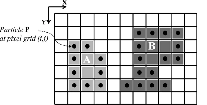
Inspired by discrete level-set methods [25], and motivated by the wish to delineate different objects in an image as individual regions, Cardinaleet al.[15] presented a discrete deformable model where the contour is represented by computational particles placed on the pixel grid. This is illustrated inFig 1and provides a geometry representation that is both explicit and implicit [25]. During the iterative segmentation process, the particles migrate to neighboring pixels and hence deform the contour. This migration is driven by an energy-minimization flow. Additional topological constraints ensure that contours remain closed and/or connected. The algorithm is a discrete version of Region Competition [26], which converges to a locally optimal solution. It is calledDiscrete Region Competition(DRC), since particles from adjacent regions compete for ownership over pixels along common boundaries.

The algorithm partitions a digital image domainOZd_{(the dimensiond= 2 or 3) into a}

background (BG) regionX0and (M−1)>0 disjoint foreground (FG) regionsXi,i= 1, ,M −1, bounded by contoursΓi,i= 1, ,M−1 [15].

FG regions are constrained to be connected sets of pixels. The void space around the FG regions is represented by a single BG region, which need not be connected. Connectivity in the FG regions is defined by a face-connected neighborhood, i.e., 4-connected in 2D and 6-con-nected in 3D. The BG region then has to be 8-con6-con-nected in 2D and 18 or 26-con6-con-nected in 3D [27]. Imposing the topological constraint that FG regions have to be connected sets of pixels regularizes the problem to the extent where the number of regions can be jointly estimated with their photometric parameters and contours [15].

The evolving contour is represented by computational particles as shown inFig 1. The algo-rithm advances multiple particles simultaneously in a processing order that does not depend on particle indexing. This ensures convergence to a result that is independent of the order in which particles are visited. Connectedness of the evolving contours is ensured by topological

Fig 1. Illustration of 2 regions (A, light gray and B, dark gray) in a 2D digital image (grid).Pixels in the background region are white. Particles are shown as black filled circles. They represent the regions by marking their outlines. Shaded pixels without a particle are interior points of the respective region.

control. The motion of the particles is driven by a discrete energy-minimization flow that locally minimizes the segmentation energy functional [15]:

E_¼E

dataþlElengthþaEmerge: ð1Þ

Here,λ_andα_{are regularization parameters trading off the weights of the contour-length and}

region-merging priors. Thefirst term measures how well the current segmentationfits (or explains) the image. The specific forms of the three terms depend on the image model, imaging model, and object model used [15].

The above energy is minimized by approximate gradient descent. The gradient is approxi-mated by the energy difference incurred by a particle move. Particles are then moved in order of descending energy reduction using a rank-based optimizer, hence ensuring that the result is independent of particle ordering [15]. Since regions may dynamically fuse and split during energy minimization, the algorithm is able to detect and segment a previously unknown and arbitrary number of regions.

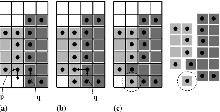
The algorithm starts from an initialization (frequently: local intensity maxima or an initial thresholding) and then refines the segmentation in iterations until no further improvement can be achieve by any particle move. In each iteration, every particle finds the set of adjacent pixels it could potentially move to. It then computes the energy differences of all possible moves. Moves that lead to topological violations are pruned from the list. Then, a graph of causally dependent moves is constructed. An example of causal dependency is illustrated inFig 2, where the possible moves of particlepdepend on the move of particleq. Assume that the energetically most favorable move for particlepis downward (Fig 2a). If the energetically most favorable move of particleqis to go left (Fig 2b), this violates the topological constraint that

Fig 2. Illustration of causally dependent moves.Assume that the energetically most favorable moves are for particlepto move down (a) and particleqleft (b). If both moves are executed, the light gray region is not connected any more, hence violating the topological constraint (c). The moves of the two particles hence causally depend on each other.

doi:10.1371/journal.pone.0152528.g002

the light-gray region has to be a 4-connected set of pixels (Fig 2c). Simply executing the ener-getically most favorable move for each particle could hence lead to topological violations. In the situation shown inFig 2, only one of the two particles can execute its most favorable move, constraining the possible moves of the other. In the present greedy descent scheme, the move that leads to the largest energy decrease has priority.

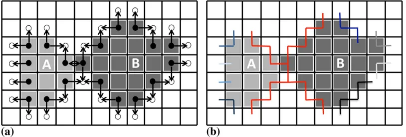
In order to find the set of moves that can be executed concurrently, we build a graph of all such causal dependencies and sort them by energy.Fig 3illustrates the construction of this undirected graph of causal dependencies. It starts from enumerating all possible moves for all particles (Fig 3a). Shrinking a region is done by removing the respective particle and inserting new boundary particles. This is irrelevant for the dependency graph. The directionality of the moves is also irrelevant and is removed, yielding a set of undirected edges. A vertex is intro-duced wherever two edges meet in any pixel. This defines the final graph (Fig 3b). Moves that are connected by a path in the graph are causally dependent. Connected sub-graphs of the final graph (highlighted by different colors inFig 3b) hence correspond to dependent sets of moves. They can extend across several particles, defining long-range chains of dependency.

Each maximal connected sub-graph can be processed independently. While the moves within a maximal connected sub-graph are causally dependent, there are no dependencies across different maximal connected sub-graphs. In order to find the energetically most favor-able set of moves that can be executed simultaneously, the edges in each maximal connected sub-graph are sorted by energy difference. In each sub-graph, the move that leads to the largest decrease in energy is executed.

Splits and fusions of FG regions are topological changes that are allowed by the energy. They are detected using concepts from digital topology [15,25,27–29] and accepted if energet-ically favorable. The BG region is allowed to arbitrarily change its topology.

Data distribution by domain decomposition

We parallelize the DRC algorithm in a distributed environment by applying a domain-decom-position approach to the image. The input image is decomposed into disjoint sub-images that

Fig 3. Illustration of the dependency graph construction.(a) All possible moves are enumerated for all particles. (b) The undirected graph of causal dependencies is obtained by removing directionality and joining edges that share a common pixel. The maximal connected sub-graphs are represented by different colors.

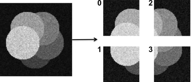
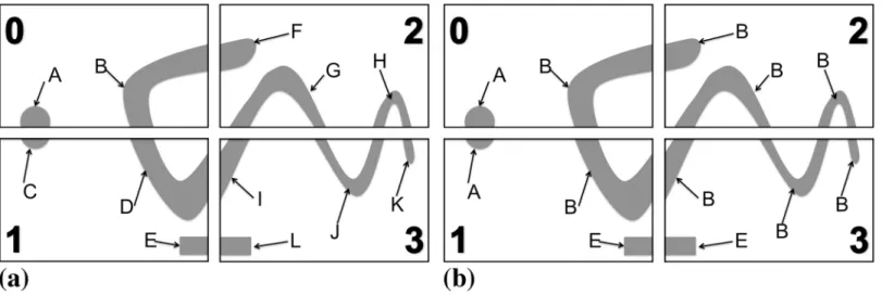
are distributed to different computers. This is illustrated inFig 4. Domain decomposition and data distribution are done transparently by the PPM library [17–19]. Reading the input image from a file is also done in a distributed way, where each computer only reads certain image planes. The PPM library then automatically redistributes the data so as to achieve a good and balanced decomposition. Each computer only stores its local sub-image, and no computer needs to be able to store the entire image data.

The algorithm is then initialized locally on each computer, using only the local sub-image. The boundary information between sub-images is communicated between the respective com-puters with ghost layers. Ghost layers are extra layers of pixels around each sub-image that rep-licate data from the adjacent sub-images on the other processors, as illustrated inFig 5. The width of these ghost layers is determined by the number of pixels required to compute energy differences, i.e., by the radius of the energy kernel (see Ref. [15] for details). The width of the ghost layer defines the communication overhead and hence the parallel scalability of the algo-rithm. PPM ghost mappings [17–19] are used to transparently update and manage ghost layer information whenever the corresponding pixels on the other computer have changed.

The initial segmentation from which the algorithm starts can be determined in a number of ways.Fig 5shows an example of an initial segmentation given by uniformly distributed circles (shown in red). From there, the algorithm evolves to the final result. Using an initialization that is so far from the final result, however, increases the runtime and also bears the risk of get-ting stuck in a sub-optimal local energy minimum. In practice, we hence usually initialize by a local-maximum detection or an initial intensity thresholding.

Starting from the initial segmentation, each FG region is identified by a globally unique label [15]. This requires care in a data-distributed setting, since different computers could use the same label to denote different regions. In our implementation, each processor first per-forms an intermediate local labeling of the regions in its sub-image. Using the processor num-ber (i.e., processor ID), this is done such that no two labels are used twice (seeFig 6a). All

Fig 4. An illustrative example showing domain decomposition and distribution of an image across four computers (numbered 0 to 3).

doi:10.1371/journal.pone.0152528.g004

regions are hence labeled uniquely. However, regions extending across more than one sub-image will be assigned multiple, conflicting labels. In a second step, the algorithm resolves these conflicts, ensuring that each FG region is uniquely labeled.

Using the definition that a FG region has to be a connected set of pixels, uniquely labeling them can be done using a parallel connected-component algorithm [30–35]. We here use the algorithm proposed by Flaniganet al.[30], which is based on an iterative relaxation process. During this, each sub-image exchanges boundary-crossing labels with neighboring processors. The labels are then replaced by the minimum of the two labels from the two processors. This process continues in iterations until a fixed point (labels do not change any more on any pro-cessor) is reached [30]. This is only done once, during initialization, and leads to a result as illustrated inFig 6b. Every FG region now has a globally unique, unambiguous label, indepen-dent of which sub-image it lies in, or across how many computers the image has been distrib-uted. This sets the basis for the energy-minimization iterations of the DRC algorithm.

Parallel contour propagation

Following initialization and initial region labeling, particles move across the image as driven by the energy-minimization flow in order to compute the segmentation. As outlined in the section

“Review of Discrete Region Competition”, this involves construction of a dependency graph of causally dependent particle moves, followed by selecting a maximal set of non-interfering moves. In a data-distributed setting, the problem occurs that every computer only knows the part of the graph that resides in its local sub-image. If graphs span across processor boundaries, correct move selection cannot be guaranteed without additional communication. This

Fig 5. Ghost layers communicate information between neighboring sub-images residing on different computers.In the example from the previous figure, processor 0 receives ghost data from processors 1, 2, and 3, as shown for a ghost layer of 10 pixels width. The same is also done on all of the other processors. This allows the particles (boundary pixels of red regions) to smoothly migrate across computers, and energy differences to be evaluated purely locally on each sub-image.

communication between computers is required to find a globally consistent set of independent moves, but should be kept to a minimum in order to guarantee algorithm scalability.

In our implementation, finding a globally consistent set of moves starts by each processorP

creating a local undirected graphGP, comprising its interior and ghost particles. Disconnected

parts of the graph that entirely lie within the local sub-image are calledinterior sub-graphs Gi P.

Parts of the graph that extend across sub-image boundaries are calledboundary sub-graphs Gb P.

Identifying compatible moves in an interior sub-graph can be done independently by each processor. Resolving boundary sub-graphs, however, requires information from all sub-images across which the sub-graph extends. This is challenging because the sub-graphs sizes, struc-tures, and distributions are not knowna priori, as they depend on the input image data.

Traditionally, master-slave approaches have been used to solve this problem on distributed machines. This is illustrated inFig 7. In this approach, the boundary sub-graphsGb

Pfrom all

processors are gathered on one single processor, the master processor. This master processor then determines the move sets and sends them back to the respective other processors. Mean-while, the other processors work on their interior sub-graphs.

This approach is easy to implement, but carries substantial overhead due to the global com-munication and the task serialization on the master processor. As we show below, this

approach does not scale and prevents acquisition-rate image analysis.

We address this problem by introducing a new parallel contour propagation algorithm, which does not require global communication and incurs no serialization. In theory, it hence scales perfectly. Instead of gathering all boundary sub-graphsGb

Pon one master processor, we

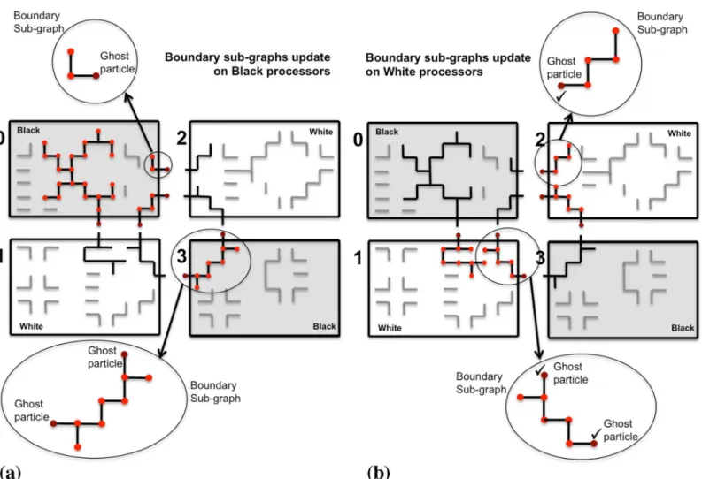
propose to use the locally available boundary sub-graph on each processor and identify the compatible moves only on that local part. If all processors did this in parallel, however, confl ict-ing moves across sub-image boundaries would occur. We avoid this by decomposict-ing the pro-cessors into two sets: black and white propro-cessors. Since FG regions are face-connected, using a checkerboard decomposition as illustrated inFig 8ensures that boundary sub-graphs always cross from black to white processors, or vice versa. They never cross sub-image boundaries within one color, hence avoiding boundary conflicts if the processing is done by color. There-fore, the black processors start by determining the viable moves on their boundary sub-graphs,

Fig 6. Region label initialization starts by each processor assigning unique labels to the FG regions in its sub-image (a).This, however, leads to conflicts for regions extending across multiple sub-images, as they will receive multiple, conflicting labels. Using a parallel connected-component algorithm [30], these conflicts are resolved in a second step, leading to a globally unique label for each FG region (b).

doi:10.1371/journal.pone.0152528.g006

while the white processors work on their interior sub-graphs. Then, the black processors com-municate their boundary decisions to the neighboring white processors using a ghost particle mapping [17]. Finally, the white processors resolve their boundary sub-graphs using the received decisions as boundary conditions, while the black processors work on their interior sub-graphs. This procedure is illustrated inFig 8. It effectively avoids conflicts and determines a globally viable move set within two rounds of local ghost communication.

Taking advantage of non-blocking MPI operations, the whole procedure is executed in an asynchronous parallel way, as detailed in Algorithm 1. This largely hides the communication time of the ghost mappings, resulting in better scalability and speed-up on a distributed mem-ory parallel machine.

Algorithm 1: Parallel distributed-memory contour propagation algorithm

Find: interior and boundary maximal connected sub-graphs,Gi PandG

b P

ifBlack processorthen

Receive: ghost information from white neighbor processors

foreachboundary sub-graphGb Pdo

identify compatible moves

Send: non-blocking send of updated boundary particle information to white neighbor processors

foreachinterior sub-graphsGi Pdo

identify compatible moves

Wait: for non-blocking send to complete

ifWhite processorthen

Send: non-blocking send of boundary particle information to black neigh-bor processors

Receive: non-blocking receive of ghost information from black neighbor processors

foreachinterior sub-graphGi Pdo

identify compatible moves

Wait: for non-blocking receive to complete

foreachboundary sub-graphsGb Pdo

identify compatible moves under ghost constraints

Fig 7. The master-slave approach to finding the global independent move set by gathering all boundary sub-graphs on a single master processor and then sending back the results.In this example, processor 0 is the master.

Breaking the boundary sub-graphs along sub-image boundaries changes the sorting order of compatible moves, and hence the convergence trace of the algorithm in energy space. Enforcing boundary conditions at the break points of the boundary sub-graphs amounts to an approximation of the original problem. This approximation is not guaranteed to determine the same global move set as the sequential approach, because the moves are only sorted by energy locally in each sub-graph, and not globally in the entire graph. However, as long as the statisti-cal distribution of break points in the graph is unbiased, the optimizer is still guaranteed to converge, albeit the path of convergence may differ. This is a famous result from Monte Carlo (MC) approaches to the Ising model [36], where it has been shown that unbiased randomiza-tion of the moves may even accelerate convergence toward an energy minimum. In our case, the distribution of break points is indeed unbiased. This is because it is the result of a domain decomposition that depends on the number of processors used, and the graphs depend on the

Fig 8. Distributed sub-graph algorithm to determine a globally consistent set of particle moves.The processors are divided into black and white ones using a checkerboard decomposition. (a) Compatible moves are identified simultaneously on all boundary sub-graphs (black) on the black processors, while the white processors work on their interior sub-graphs (gray). (b) Boundary particles (dark red) are send from the black to the white processors in order to provide the boundary condition for the boundary sub-graph processing on the white processors. The ghosts are not altered by the white processors, but immediately accepted as moves (symbolized by the check marks). This avoids conflicts and only requires local communication.

doi:10.1371/journal.pone.0152528.g008

unpredictable image content. Therefore, independent unbiased breaking is satisfied, and the distributed approach converges.

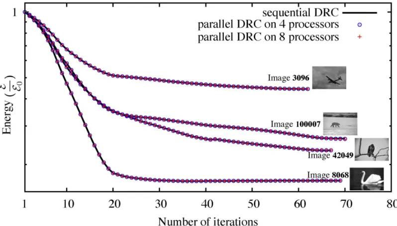
We empirically confirm this convergence by comparing the energy evolution of the original sequential algorithm [15] and our new distributed method on different 2D benchmark images from the Berkeley database [37]. The result for four example images is shown inFig 9using dif-ferent numbers of processors and hence difdif-ferent sub-graph decompositions. In all tested cases, both methods converge. The largest observed difference in final energy is less than 0.5%.

Fig 10shows histograms of the energy differences for 25 images from the Berkeley database. Three metrics are shown: (a) the maximum energy difference occurring anywhere along the convergence path, (b) the difference in the energy of the final converged state, (c) the difference in the number of iterations requires to reach convergence.

The results in Figs9and10show that the parallel algorithm is in good agreement with the original sequential algorithm [15]. Both algorithms show the same energy-evolution trend and converge to almost the same energy level with less than 0.5% difference anywhere during energy evolution.Fig 10calso confirms the Ising-model result that the randomized parallel algorithm on average converges in fewer iterations than the sequential method.

The question arises, however, if these small energy differences are significant in terms of the final segmentation. While no general guarantee can be given, the final segmentations were

Fig 9. Energy evolution of the sequential DRC algorithm [15] and the present parallel algorithm on four different images from the Berkeley database [37] on 4 and 8 processors.Despite the boundary sub-graph decomposition (see main text), the results are pixel-wise identical in all cases except for image 100007, where two pixels on 4 processors and 3 pixels on 8 processors differ from the sequential result due to contour oscillations, as discussed in the main text.

close in all cases tested, with at most 3 pixels differing between the sequential and parallel solu-tions. All observed pixel differences stemmed from contour oscillations around the converged state, as confirmed by pixel-wise comparison of the final segmentations. These oscillations are an inherent property of the energy descent method used in DRC [15]. They are suppressed by reducing the number of concurrently accepted moves whenever oscillations occur [15]. This is required in order to guarantee convergence of DRC. In our distributed DRC implementation, oscillations are detected locally by each computer. Also, the number of accepted moves per iter-ation is set locally, and potentially differently, by each computer. The oscilliter-ation pattern close

Fig 10. Comparison of the results from the distributed DRC algorithm and the original sequential implementation [15] on 25 2D images from the Berkeley benchmark database [37].(a) Histogram of the maximum energy difference occurring anywhere along the energy evolution path;E_DRCis the sequential algorithm andE_Nthe distributed algorithm onNcomputers. (b) Histogram of thefinal energy difference of the converged solutions. (c) Histogram of the difference in the total number of iterations required to reach the convergedfinal solution.

doi:10.1371/journal.pone.0152528.g010

to the final converged state is hence different than the one in sequential DRC. An example is shown inFig 11where the only differences between the two segmentations are the two oscil-latory particles shown in white. Since they may stop their oscillations at different locations, the final segmentations may differ in these two pixels, which explains the small energy difference. The final segmentations are, however, geometrically close, and the algorithm converges toward the same local energy minimum. It is also important to keep in mind that the sequential DRC algorithm uses an approximate local optimizer that may not find the globally best segmenta-tion. Sometimes, the slightly different result obtained by the distributed method is therefore better in terms of energy (seeFig 10b).

Parallel topology processing and data-structure update

After having determined the set of compatible acceptable moves, the particles (and hence the contours) propagate in parallel on each processor. This changes the region labels of the corre-sponding pixels, as regions move, shrink, or grow. Particles that move across sub-image bound-aries are communicated to the respective destination processor using the local neighborhood mappings of PPM [17]. This ensures global consensus about the propagating contours.

In addition to propagating, contours can also split or fuse if that is energetically favorable. This corresponds to a region splitting into two, or two regions merging. While digital topology allows such topological changes in the segmentation to be efficiently detected using only local information [15], the labels of the involved regions may change across sub-image boundaries. Whenever region labels change as a result of a split or fusion, a seeded flood-fill is performed in the original DRC algorithm [15], in order to identify the new connected components. This again requires additional care in a distributed setting, as illustrated inFig 12.

Fig 12ashows the two critical situations: two regions touching at a sub-image boundary that are not supposed to fuse (by the image energy model) and a split in a region that extends across multiple sub-images. The parallel connected component algorithm [30] used during initializa-tion would unnecessarily re-label all regions that cross any sub-image boundary and errone-ously fuse the two touching regions (Fig 12b). In order to obtain the correct result, we propose a particle-based alternative, as detailed in Algorithm 2.

Fig 11. The small energy differences between the distributed and the sequential DRC implementations result from local pixel oscillations.An example is shown with a synthetic image using a piecewise smooth image model for segmentation. (a) Result on a single computer. (b) Result from the distributed algorithm on 8 computers. (c) Overlay of the two results with differences shows in white. These are two oscillatory particles jumping back and forth between two neighboring pixels. The final segmentation results are hence very close and amount to alternative pixelations of the object border line.

Algorithm 2: Distributed region re-labeling

Reconstruct: label imageL

hotpart false

Create an empty list S

ifcontour particle label changes at sub-image boundarythen

activate particle as a hot particle

hotpart true

Ghost mappings: Particle

ifthere is any hot ghost particlethen

add it as a seed to the listS Global: reduce operation onhotpart whilehotpartdo

Reconstruct label imageLusing flood fill from the seeds inS Empty:S

Ghost mappings: Particle

ifthere is any hot ghost particlethen

add it as a seed to the listS

Fig 12. Distributed region split and merge algorithm.In the upper row, the evolving contours are shown by dashed lines and the underlying objects to be segmented by the black solid regions. (a) The situation before re-labeling the regions. Two regions (B/C) touch at a sub-image boundary, but should not fuse according to the image energy model. The region A extends across multiple sub-images and splits in sub-image 3. (b) Applying a parallel connected-component algorithm [30] would erroneously fuse regions touching at sub-image boundaries and unnecessarily re-label all regions with new unique labels.

doi:10.1371/journal.pone.0152528.g012

which we call“hot particles”from now on, as inspired by the classical forest-fire algorithm, are then sent to the neighboring processor.

The neighboring processor receiving the hot ghost particles starts a local forest-fire algo-rithm for seeded flood filling of the region, using the hot ghosts as seeds. Since this may propa-gate the label change across multiple processors, the procedure proceeds in iterations until no more hot particles are detected anywhere. This is determined by a global all-reduce operation of local flags for the presence of hot particles in each sub-image. Regions are always re-labeled using the lower of the two labels. This means that hot particles only propagate changes with new labels lower than existing ones. Therefore, the procedure is guaranteed to terminate, as oscillations or loops cannot occur.

The complete procedure is detailed in Algorithm 2. Again, all communication (mappings) is done asynchronously using non-blocking MPI operations. After execution of the algorithm, all regions are again identified by globally unique labels, but only necessary changes are made. Regions that did not undergo topological changes retain their previous labels. This prevents spurious region fusions and keeps the data-structure updates to a minimum. Also,

Fig 13. Boundary particles are activated upon region label changes in the local sub-image.Only activated (“hot”) boundary particles are communicated to the neighboring processor, restricting re-labeling to affected regions and avoiding communication of a full ghost layer of pixels. (a) All boundary particles (black disks) are deactivated (“cold”) before local region label update. (b) Boundary particles of re-labeled regions are activated (red disks,

“hot”) and propagate the label change to the neighboring processor.

communicating only hot ghost particles, instead of full pixel layers, significantly reduces the communication overhead.

Results

We first show correctness and efficiency of the distributed parallel algorithm and then illustrate its application to acquisition-rate image segmentation in 3D light-sheet fluorescence micros-copy. We demonstrate correctness by comparison with the original reference implementation of Cardinaleet al.[15] on synthetic and real-world images taken from the original DRC paper [15]. Then, we assess the parallel efficiency and scalability of the present implementation using scalable synthetic images in both a weak-scaling and a strong-scaling experiment.

All computations were performed using the PPM library [17–19] in its 2015 version on the Bull cluster“taurus”at the Center for Information Services and High Performance Computing (ZIH) of TU Dresden. The cluster island used consists of 612 Intel Haswell nodes with 24 cores per node and 2.5 GB of main memory per core. The parameter settings for all test cases are summarized inTable 1. They were determined following the guidelines given in the original DRC publication [15].

Correctness of the distributed algorithm

Results using a piecewise constant image model. We first check that the distributed

algo-rithm produces the same results as the sequential benchmark implementation in the case of a multi-region piecewise constant (PC) image model. In this model, the assumption is that differ-ent FG regions have differdiffer-ent intensities that are, however, spatially constant within each

Table 1. Parameter settings used for the cases shown in this paper (PC: piecewise constant; PS: piecewise smooth).See Ref. [15] for parameter meaning and guidelines.

Initialization Algorithm parameters E

data Energy parameters

Icecream PC 2D, 130 × 130,Fig 14

6 × 6 bubbles θ= 0.02,Rκ= 4 PC λ= 0.04

Bird, 481 × 32,Fig 16

32 × 21 bubbles θ= 4.5,Rκ= 5 PC λ= 0.2

Cell nuclei, 672 × 512,Fig 17

local maxima θ= 0.02,Rκ= 4 PC λ= 0.06

Icecream PS 2D, 130 × 130,Fig 18

5 × 5 bubbles θ= 0.2,Rκ= 4 PS λ= 0.04,β= 0.05,R= 8

Elephants 2D, 481 × 321,Fig 20

21 × 14 bubbles θ= 0.2,Rκ= 8 PS λ= 0.2,β= 0.05,R= 4

Zebrafish embryo germ cells 3D, 188 × 165 × 30,Fig 21

bounding box Rκ= 4 PS λ= 0.08,β= 0.005,R= 9μm

Synthetic unit cell test image 3D, 256 × 256 × 256,Fig 22

local maxima θ= 0.02,Rκ= 4 PC λ= 0.04

Drosophila embryo 3D, 1824 × 834 × 809,Fig 25

local maxima from blob detector θ= 0.001,Rκ= 8 PC λ= 0.005

Drosophila embryo 3D, 1824 × 834 × 809,Fig 26

local maxima from blob detector θ= 0.001,Rκ= 8 PS λ= 0.005,β= 1.0,R= 8

zebrafish vasculature 3D, 1626 × 988 × 219,Fig 27

thresholding θ= 10.0,Rκ= 8 PS λ= 0.02,β= 0.001,R= 12

doi:10.1371/journal.pone.0152528.t001

one and four processors produces the exact same result as the benchmark implementation. As a second real image, we consider the same fluorescence microscopy image of nuclei as in the original publication [15]. The results on one and 16 processors are shown inFig 17. The algorithm is initialized with a circular region around each local intensity maximum after blur-ring the image with a Gaussian filter of widthσ= 10 pixel. This is the same initialization as

used in Ref. [15]. The results are identical, pixel by pixel.

Results using a piecewise smooth image model. The DRC algorithm is generic over a

wide range of image models, including the more complex piecewise smooth (PS) model. In this model, each region is allowed to have a smooth internal intensity shading. We again use the same synthetic test image as in Ref. [15] and illustrate the result inFig 18. Pixel-to-pixel com-parison of the final segmentation results shows differences in two oscillatory pixels on eight processors (see alsoFig 11). This is consistent with the way boundary oscillations are detected and handled in the distributed algorithm in comparison with the sequential one.

The energy evolution for this case is shown inFig 19in comparison with the original sequential DRC algorithm of Cardinaleet al.[15]. Again, the two convergence traces are almost identical with small differences stemming from the graph decomposition used in the present implementation. The difference in final energy is due to the two oscillatory pixels, as discussed above and shown inFig 11.

Fig 20illustrates the sequential and distributed segmentations of a natural-scene image using the PS image model. By pixel-to-pixel comparison, the segmentation result on four pro-cessors (Fig 20d) is identical to the one computed by a single computer (Fig 20b).

As a first 3D test image, we use the same fluorescence confocal image of zebrafish germ cells that was also used in Ref. [15].Fig 21shows the raw image along with the PS segmentation results on one and four processors. By pixel-wise comparison, the results are identical.

Efficiency of the distributed algorithm

Fig 14. Distributed segmentation of a synthetic test image using a piecewise constant image model.(a) Initialization on a single processor with particles shown in red. (b) Final result on a single processor. (c) Initialization on four processors. (d) Final result on four processors. (e) Initialization on eight processors. (f) Final result on eight processors. The results are identical to those in Ref. [15] in all cases.

contents. Moreover, synthetic images can easily be scaled to arbitrary size, as required for the weak scaling tests.

The two synthetic images used here are shown inFig 22. These are 3D images, andFig 22

shows maximum-intensity projections. The top row inFig 22shows the“unit cells”, from which the test images are generated by periodic concatenation as shown in the panels below. In the first image (Fig 22a), all objects are local, i.e., there are no objects that cross sub-image boundaries. The second image (Fig 22b) contains objects that cross sub-image boundaries. Comparing the results of the two allows us to estimate the communication overhead from the parallel graph-handling and region labeling algorithms introduced here. In all cases, the algo-rithm is initialized with circular regions around each local intensity maximum after blurring the image with a Gaussian filter ofσ= 5 pixel.

In the weak scaling, the workload per processor remains constant, while the overall image size increases proportionally to the number of processors. This way, the workload on 512 pro-cessors is an image of 8192 × 4096 × 256 pixels containing 18 944 objects. Periodically repeat-ing the“unit cell”image, rather than scaling it, ensures that the workload on each processor is exactly the same, since every processor locally“sees”the same image.

Fig 15. Energy evolution of the sequential DRC algorithm of Cardinaleet al.[15] in comparison with the present distributed algorithm processing the piecewise constant test image fromFig 14on four and eight processors.

Fig 23shows the resulting parallel efficiency (weak scaling) for the two test images. For com-parison, it also shows the parallel efficiency when using the classical master-slave approach to graph processing (seeFig 7). This approach does not scale, as the parallel efficiency rapidly drops when using more than 32 processors. This results from the communication overhead due to global communication, and from the additional serialization. The present randomized approach scales for both test images.

Segmentation of the second data set using the present parallel approach on 1, 64, and 512 processors took less than 12, 24, and 29 seconds respectively, corresponding to image sizes of 32 MB, 2 GB, and 16 GB, respectively, in this weak-scaling test. Comparing the results for the first test image, where no objects cross sub-image boundaries, with those for the second test image reveals that about half of the communication overhead is due to boundary particles.

Strong scaling measures how efficiently a parallel algorithm reduces the processing time for an image of a given and fixed size by distributing it across an increasing number of processors.

Fig 16. Distributed segmentation of a natural-scene image using a piecewise constant image model.(a) Initialization on a single processor with particles shown in red. (b) Final result on a single processor. (c) Initialization on four processors. (d) Final result on four processors. The results are identical to those in Ref. [15] in both cases.

doi:10.1371/journal.pone.0152528.g016

Fig 18. Parallel segmentation of a synthetic image using a piecewise smooth image model.(a) Initialization on a single processor with particles shown in red. (b) Final result on a single processor. (c) Initialization on four processors. (d) Final result on four processors. (e) Initialization on eight processors. (f) Final result on eight processors. Two oscillatory pixels differ with respect to the result in Ref. [15] (see alsoFig 11).

Since the workload per processor decreases as the number of processors increases in a strong scaling, the relative communication overhead steadily grows. Strong scalability is hence always limited by problem size with large problems scaling better. We therefore show tests for two dif-ferent image sizes: a moderate image size of 512 × 512 × 512 pixels (black circles inFig 24) and a large image of 2048 × 2048 × 2048 pixels (red squares inFig 24).

For the first image of size 512 × 512 × 512 pixel, the decrease in efficiency beyond 8 proces-sors is due to communication between the procesproces-sors, which increases relatively to the smaller and smaller computational load per processor. A 30-fold speedup is achieved for this image size on 64 processors. On 512 processors, every processor only has a sub-image of size 64 × 64 × 64 pixel with ghost layers of width 5 pixel all around. Segmentation of this image on 8, 64, and 512 processors took 16, 4.2, and 1.6 seconds, respectively.

For the larger image of size 2048 × 2048 × 2048 pixel, segmentation on one processor is not possible, since it would require 62 GB of main memory. On 8 and more processors, segmenta-tion becomes feasible and takes 6870 seconds on 8 processors. On 64 and 512 processors, the result is computed in 860 and 145 seconds, respectively. A 48-fold speed is achieved on 512 processors relative to 8 processors, which corresponds to a scalability close to the optimal line.

Fig 19. Energy evolution of the sequential DRC algorithm of Cardinaleet al.[15] in comparison with the present distributed algorithm processing the piecewise smooth test image fromFig 18on four and eight processors.

Application to acquisition-rate segmentation of 3D light-sheet

microscopy data

We present case studies applying the present algorithm to segmenting 3D image data from light-sheet microscopy, demonstrating that acquisition-rate segmentation is possible. We use images of stained nuclei and of vasculature in order to demonstrate the flexibility of the method to segment different shapes.

The first image shows a whole liveDrosophila melanogasterembryo at cellular blastoderm stage with nuclei labeled by a histone marker. This data was acquired on an OpenSPIM micro-scope [38] in the Tomancak lab at MPI-CBG. The size of the original image file is 4.6 GB at 32 bit depth. The image has 1824 × 834 × 809 pixels. During the segmentation, a total of about 64 GB of main memory is required for DRC. Distributed across 128 processors, this is 500 MB per processor, which fits the memory of the individual cores. The segmentation results using the present distributed algorithm with the PC image model on 128 processors is shown inFig 25c.

Fig 20. Distributed segmentation of a natural-scene image using a piecewise smooth image model.(a) Initialization on a single processor with particles shown in red. (b) Final result on a single processor. (c) Initialization on four processors. (d) Final result on four processors. The two results are identical.

doi:10.1371/journal.pone.0152528.g020

Fig 21. Distributed segmentation of zebrafish primordial germ cells using a piecewise smooth image model.(a) Raw 3D confocal fluorescence microscopy image showing three cells with a fluorescent membrane stain (image: M. Goudarzi, University of Münster). (b) Segmentation result on a single processor. (c) Segmentation result on four processors. The two results are identical.

Fig 25eshows the sub-image from one of the processors, andFig 25fthe corresponding part of the segmentation result. Communication across sub-image boundaries ensures that the pro-cessors collectively solve the global problem without storing all of it.

Segmenting this image distributed across 128 processors took less than 60 seconds, which is shorter than the time of 90 seconds until the microscope acquires the next time point. We hence achieve acquisition-rate image segmentation in this example, using a state-of-the-art model-based segmentation algorithm that produces high-quality results. If necessary, more

Fig 22. Maximum-intensity projections of the synthetic test images used to assess the parallel performance and scalability of the distributed algorithm.(a) 256 × 256 × 256 pixel unit cell of the first test image where no object touches or crosses the boundary. The image contains 37 ellipsoidal objects of different intensities. All objects are non-overlapping in 3D, even though they may appear overlapping in the maximum projection shown here. (b) 256 × 256 × 256 pixel unit cell of the second test image with objects touching and crossing the boundary. The image contains 48 ellipsoidal objects of different intensities. The object number is higher than in the first image, because some objects are partial, but the fraction of FG pixels vs. BG pixels is the same as in (a) in order to keep the computational cost (i.e., the number of particles) constant. (c) Synthetic workload image of type 1, generated from 4 unit cells by periodically concatenating them. (d) Synthetic workload image of type 2, generated from 4 unit cells by periodically concatenating them.

doi:10.1371/journal.pone.0152528.g022

processors can be used to further reduce processing time, as we have shown the present imple-mentation to scale well up to 512 processors.

We compare our approach with the TWANG [10] pipeline on 14 cores of one compute node (TWANG does shared-memory multi-threading). TWANG [10] required 24 minutes to compute the segmentation using the 14 cores, which does not allow acquisition-rate process-ing. The comparison is mainly in terms of computational performance, since TWANG was optimized for segmenting spherical objects, whereas the nuclei in our image are rather elon-gated. The result from DRC hence shows better segmentation quality.

Due to the inhomogeneous fluorescence intensity across the sample, the PC segmentation shown inFig 25cmisses some of the nuclei at the left tip of the embryo. This can be improved using the PS image model instead, which allows for intensity gradients within regions, in par-ticular within the background region. This is shown inFig 26.Fig 26ashows a low-intensity

Fig 23. Weak scaling parallel efficiency of the present method in comparison with the classical master/slave approach.Timet1is the runtime of the algorithm to process a“unit cell”image on one processor, andtPis the runtime to segment aP-fold larger periodic concatenation image distributed overP processors. The images on 1 to 16 processors are shown below the abscissa for illustration.

region where the PC model misses some nuclei.Fig 26bshows a high-intensity regions where the PC model fuses several nuclei together. The corresponding results when using the PS image model are shown in the panels below, inFig 26c and 26d. The whole-image result when using the PS image model is shown inFig 26e. The PS model improves the segmentation since it adjusts to local intensity variations in the objects and the background, which is also why it cap-tures more of the fiducial beads around the embryo. This demonstrates the flexibility of DRC to accommodate for different image models, enabling application-specific segmentations that include prior knowledge about the image. The segmentation quality can further be improved by including shape priors [23,40], as has been demonstrated for DRC [41], or by using Sobolev gradients for which DRC is uniquely suited [42].

Using the PS image model, however, is computationally more involved than using the PC model. The segmentation shown inFig 26erequired 250 seconds to be computed on 128 pro-cessors. Acquisition-rate processing using the PS model hence requires about 512 propro-cessors. The second image shows the tail of a live zebrafish embryo 3.5 days post fertilization with the vasculature fluorescently labeled by expressing GFP in endothelial cells (Tg(flk1:EGFP) s843). This image was acquired by the Huisken lab at MPI-CBG using a state-of-the-art light-sheet microscope [1]. The geometric structure of a vascular network is very different from blob-like nuclei, illustrating the flexibility of DRC to segment arbitrary shapes. This image is

Fig 24. Strong scaling speedup versus number of processorsPfor two different image sizes of 512 × 512 × 512 pixel (black circles) and 2048 × 2048 × 2048 pixel (red squares).The two images are shown in the insets.

doi:10.1371/journal.pone.0152528.g024

intractable for specialized blob-segmentation pipelines like TWANG [10].Fig 27ashows the raw data. The image has 1626 × 988 × 219 pixels.Fig 27bshows the segmentation result using Li’s minimum cross-entropy thresholding [43], as implemented in the software packageFiji

[44]. We use this thresholding as an initialization for our method.Fig 27cis the segmentation result using the PS image model with a Gaussian noise model. Distributed processing on 32 processors took 248 seconds. In this segmentation, some vessels appear non-contiguous and the caudal vessels (caudal artery and caudal vein) are not properly resolved. This changes when replacing the Gaussian noise model with a Poisson noise model [45], as shown inFig 27d. Using the correct noise model clearly improves the result, providing further illustration that flexible frameworks like DRC are important. The result inFig 27dwas obtained on 32 proces-sors in less than 200 seconds.

Discussion

We have presented a distributed-memory parallel implementation of the Discrete Region Competition (DRC) algorithm [15] for image segmentation. Efficient parallelization was made possible by a novel parallel independent sub-graph algorithm, as well as optimizations to the parallel connected-component labeling algorithm. The final algorithm was implemented using the PPM library [17–19] as an efficient middleware for parallel particle-mesh methods. The parallel implementation includes both piecewise constant (PC) and piecewise smooth (PS) image models; it is open-source and freely available from the web page of the MOSAIC Group and from github:https://github.com/yafshar/PPM_RC.

The distributed-memory scalability of the presented approach effectively overcomes the memory and runtime limitations of a single computer. None of the computers or processors over which a task is distributed needs to store the entire image. This allows segmenting very large images. The largest synthetic image considered here had 1.71010pixels, corresponding to 32 GB of uncompressed memory. A real-world light-sheet microscopy image of 1824 × 834 × 809 pixels (amounting to 4.6 GB of uncompressed memory) was segmented in under 60 sec-onds when distributed across 128 processors. This was less than the 90 secsec-onds until the micro-scope acquired the next time point, hence providing online, acquisition-rate image analysis. This is a prerequisite for smart microscopes [5] and also enables interactive experiments.

We have demonstrated the parallel efficiency and scalability of the present implementation using synthetic images that can be scaled to arbitrary size. We have further reproduced the benchmark cases from the original DRC paper [15] and shown that the parallel tion produces the same or very close results as the original sequential reference implementa-tion. Small differences may occur, but are limited to isolated oscillatory pixels, which are due to local oscillation detection. This local detection is preferable because it avoids global communi-cation and improves parallel scalability with respect to the traditional master/slave approach.

Although our performance figures are encouraging, there is still room for further improve-ments. One idea could be to compress the particle and image data before communication. This would effectively reduce the communication overhead and improve scalability. Furthermore,

Fig 25. Application of the present implementation to acquisition-rate segmentation of a 3D light-sheet microscopy image using a piecewise constant (PC) image model.All 3D visualizations were done usingClearVolume[39]. (a) Raw image showing aDrosophila melanogasterembryo at cellular blastoderm stage with fluorescent histone marker (image: Dr. Pavel Tomancak, MPI-CBG). In addition to the nuclei, there are fluorescent beads embedded around the sample as fiducial markers for multi-view fusion and registration [3]. (b) Segmentation result using the present distributed implementation of DRC with the PC image model distributed across 128 processors. The total time to compute the segmentation was 60 seconds, while the microscope acquired a 3D image every 90 seconds. (c) Example of a sub-image from one of the processors. (d) Corresponding part of the segmentation as computed by that processor.

doi:10.1371/journal.pone.0152528.g025

amount of particles. This causes asynchronous waiting times that may limit scalability. Due to the checkerboard decomposition used in the graph handling, however, the present implemen-tation is limited to Cartesian domain decompositions, while spatially adaptive trees might be better. Lastly, the local evaluation of energy differences for all possible particle moves can be accelerated by taking advantage of multi-threading and graphics processing units (GPUs). This is possible for DRC, as has already been shown [46], suggesting that processing could be further accelerated by a factor of 10 to 30, depending on the image model.

This leaves ample opportunities for further reducing processing times as required by the microscopy application. Already the present implementation, however, illustrates the algorith-mic concept, which is based on randomized graph decomposition and hybrid particle-mesh methods. This enables acquisition-rate segmentation of 3D fluorescence microscopy images using different image models, opening the door for smart microscopes and interactive, feed-back-controlled experiments.

Acknowledgments

This work was supported by the Max Planck Society and by the German Federal Ministry of Education and Research (BMBF) under funding code 031A099. We thank the Center for Infor-mation Services and High Performance Computing (ZIH) at TU Dresden for generous alloca-tion of computer time. We thank Dr. Pavel Tomancak (MPI-CBG) for providing the example image ofDrosophila melanogaster, and Dr. Jan Huisken (MPI-CBG) and Stephan Daetwyler (Huisken lab, MPI-CBG) for providing the example image of zebrafish vasculature. We also thank Pietro Incardona and Bevan Cheeseman (both MOSAIC group) for many discussions.

Author Contributions

Conceived and designed the experiments: YA IFS. Performed the experiments: YA. Analyzed the data: YA IFS. Contributed reagents/materials/analysis tools: YA. Wrote the paper: YA IFS.

References

1. Huisken J, Swoger J, Del Bene F, Wittbrodt J, Stelzer EHK. Optical Sectioning Deep Inside Live Embryos by Selective Plane Illumination Microscopy. Science. 2004; 305:1007–1009. doi:10.1126/ science.1100035PMID:15310904

2. Huisken J, Stainier DYR. Even fluorescence excitation by multidirectional selective plane illumination microscopy (mSPIM). Opt Lett. 2007 Sep; 32(17):2608–2610. Available from:http://ol.osa.org/abstract. cfm?URI=ol-32-17-2608doi:10.1364/OL.32.002608PMID:17767321

4. Schmid B, Shah G, Scherf N, Weber M, Thierbach K, Campos CP, et al. High-speed panoramic light-sheet microscopy reveals global endodermal cell dynamics. Nat Commun. 2013 Jul; 4. 00013. Avail-able from:http://dx.doi.org/10.1038/ncomms3207

5. Scherf N, Huisken J. The smart and gentle microscope. Nat Biotechnol. 2015 08; 33(8):815–818. doi: 10.1038/nbt.3310PMID:26252136

6. Amat F, Lemon W, Mossing DP, McDole K, Wan Y, Branson K, et al. Fast, accurate reconstruction of cell lineages from large-scale fluorescence microscopy data. Nat Methods. 2014 Sep; 11(9):951–958. doi:10.1038/nmeth.3036PMID:25042785

7. Caselles V, Kimmel R, Sapiro G. Geodesic active contours. Int J Comput Vis. 1997; 22(1):61–79. doi: 10.1023/A:1007979827043

8. Beare R, Lehmann G. The watershed transform in ITK—discussion and new developments. The Insight Journal. 2006 06; Available from:http://hdl.handle.net/1926/202

9. Al-Kofahi Y, Lassoued W, Lee W, Roysam B. Improved Automatic Detection and Segmentation of Cell Nuclei in Histopathology Images. IEEE T Bio-Med Eng. 2010 April; 57(4):841–852. doi:10.1109/TBME. 2009.2035102

10. Stegmaier J, Otte JC, Kobitski A, Bartschat A, Garcia A, Nienhaus GU, et al. Fast Segmentation of Stained Nuclei in Terabyte-Scale, Time Resolved 3D Microscopy Image Stacks. PLoS ONE. 2014 02; 9(2):e90036. doi:10.1371/journal.pone.0090036PMID:24587204

11. Olmedo E, Calleja JDL, Benitez A, Medina MA. Point to point processing of digital images using parallel computing. International Journal of Computer Science Issues. 2012; 9(3):1–10.

12. Galizia A, D’Agostino D, Clematis A. An MPI–CUDA library for image processing on HPC architectures. J Comput Appl Mech. 2015; 273:414–427. doi:10.1016/j.cam.2014.05.004

13. Aubert G, Kornprobst P. Mathematical Problems in Image Processing. vol. 147 of Applied Mathematical Sciences. Second edition ed. Springer New York; 2006.

14. Cremers D, Rousson M, Deriche R. A Review of Statistical Approaches to Level Set Segmentation: Integrating Color, Texture, Motion and Shape. International Journal of Computer Vision. 2007; 72 (2):195–215. Available from:http://dx.doi.org/10.1007/s11263-006-8711-1

15. Cardinale J, Paul G, Sbalzarini IF. Discrete region competition for unknown numbers of connected regions. IEEE Trans Image Process. 2012; 21(8):3531–3545. doi:10.1109/TIP.2012.2192129PMID: 22481820

16. Delong A, Osokin A, Isack HN, Boykov Y. Fast Approximate Energy Minimization with Label Costs. Int J Comput Vision. 2012; 96(1):1–27. doi:10.1007/s11263-011-0437-z

17. Sbalzarini IF, Walther JH, Bergdorf M, Hieber SE, Kotsalis EM, Koumoutsakos P. PPM—A Highly Effi-cient Parallel Particle-Mesh Library for the Simulation of Continuum Systems. J Comput Phys. 2006; 215(2):566–588. doi:10.1016/j.jcp.2005.11.017

18. Awile O, Demirel O, Sbalzarini IF. Toward an Object-Oriented Core of the PPM Library. In: Proc. ICNAAM, Numerical Analysis and Applied Mathematics, International Conference. AIP; 2010. p. 1313–

1316.

19. Awile O, MitrovićM, Reboux S, Sbalzarini IF. A domain-specific programming language for particle sim-ulations on distributed-memory parallel computers. In: Proc. III Intl. Conf. Particle-based Methods (PARTICLES). Stuttgart, Germany; 2013. p. p52.

20. Ibanez L, Schroeder W, Ng L, Cates J. The ITK Software Guide.http://www.itk.org/ItkSoftwareGuide. pdf; 2005.

21. Kass M, Witkin A, Terzopoulos D. Snakes: Active Contour Models. Int J Comput Vis. 1988;p. 321–331. 22. Montagnat J, Delingette H, Ayache N. A review of deformable surfaces: topology, geometry and

defor-mation. Image and Vision Comput. 2001; 19(14):1023–1040. Available from:http://www.sciencedirect. com/science/article/pii/S0262885601000646doi:10.1016/S0262-8856(01)00064-6

23. Zhang D, Lu G. Review of shape representation and description techniques. Pattern Recognition. 2004; 37(1):1–19. Available from: doi:10.1016/j.patcog.2003.07.008

24. Xu C, Yezzi J A, Prince JL. On the relationship between parametric and geometric active contours. In: Signals, Systems and Computers, 2000. Conference Record of the Thirty-Fourth Asilomar Conference on. vol. 1; 2000. p. 483–489 vol.1.

25. Shi Y, Karl WC. A Real-Time Algorithm for the Approximation of Level-Set-Based Curve Evolution. IEEE Trans Image Process. 2008; 17(5):645–656. doi:10.1109/TIP.2008.920737PMID:18390371 26. Zhu SC, Yuille A. Region competition: Unifying snakes, region growing, and Bayes/MDL for multiband

image segmentation. IEEE Trans Pattern Anal Machine Intell. 1996 Sep; 18(9):884–900. doi:10.1109/ 34.537343

uted memory architectures. Computer Physics Communications. 2000; 130(1-2):118–129. Available from:http://www.sciencedirect.com/science/article/pii/S0010465500000461doi:10.1016/S0010-4655 (00)00046-1

33. Tiggemann D. Simulation of percolation on massively-parallel computers. International Journal of Mod-ern Physics C. 2001; 12(06):871. doi:10.1142/S012918310100205X

34. Wang Kb, Chia Tl, Chen Z, Lou Dc. Parallel execution of a connected component labeling operation on a linear array architecture. Journal of Information Science And Engineering. 2003; 19:353–370. 35. Moloney NR, Pruessner G. Asynchronously parallelized percolation on distributed machines. Phys Rev

E. 2003 Mar; 67:037701. Available from:http://link.aps.org/doi/10.1103/PhysRevE.67.037701doi:10. 1103/PhysRevE.67.037701

36. Pawley GS, Bowler KC, Kenway RD, Wallace DJ. Concurrency and parallelism in MC and MD simula-tions in physics. Comput Phys Commun. 1985; 37(1-3):251–260. doi:10.1016/0010-4655(85)90160-2 37. Martin D, Fowlkes C, Tal D, Malik J. A database of human segmented natural images and its application

to evaluating segmentation algorithms and measuring ecological statistics. In: Proc. IEEE Intl. Conf. Computer Vision (ICCV). Vancouver, BC, Canada; 2001. p. 416–423.

38. Pitrone PG, Schindelin J, Stuyvenberg L, Preibisch S, Weber M, Eliceiri KW, et al. OpenSPIM: an open-access light-sheet microscopy platform. Nat Methods. 2013 Jul; 10(7):597–598. doi:10.1038/ nmeth.2507

39. Royer LA, Weigert M, Günther U, Maghelli N, Jug F, Sbalzarini IF, et al. ClearVolume: open-source live 3D visualization for light-sheet microscopy. Nat Methods. 2015 Jun; 12(6):480–481. doi:10.1038/ nmeth.3372PMID:26020498

40. Veltkamp RC, Hagedoorn M. 4. State of the Art in Shape Matching. Principles of visual information retrieval. 2001;p. 87.

41. Cardinale J. Unsupervised Segmentation and Shape Posterior Estimation under Bayesian Image Mod-els [PhD Thesis, Diss. ETH No. 21026]. MOSAIC Group, ETH Zürich; 2013.

42. Sbalzarini IF, Schneider S, Cardinale J. Particle methods enable fast and simple approximation of Sobolev gradients in image segmentation. arXiv preprint arXiv:14030240v1. 2014;p. 1–21.

43. Li CH, Lee CK. Minimum Cross Entropy Thresholding. Pattern Recognition. 1993; 26(4):617–625. doi: 10.1016/0031-3203(93)90115-D

44. Schindelin J, Arganda-Carreras I, Frise E, Kaynig V, Longair M, Pietzsch T, et al. Fiji: an open-source platform for biological-image analysis. Nat Methods. 2012; 9(7):676–682. doi:10.1038/nmeth.2019 PMID:22743772

45. Paul G, Cardinale J, Sbalzarini IF. Coupling Image Restoration and Segmentation: A Generalized Lin-ear Model/Bregman Perspective. Int J Comput Vis. 2013; 104(1):69–93. Available from:10.1007/ s11263-013-0615-2