A review of the theoretical basis for bulk mass flux convective parameterization

www.atmos-chem-phys.net/10/3529/2010/ © Author(s) 2010. This work is distributed under the Creative Commons Attribution 3.0 License.

Chemistry

and Physics

A review of the theoretical basis for bulk mass flux

convective parameterization

R. S. Plant

Department of Meteorology, University of Reading, Earley Gate, P.O. Box 243, Reading, RG6 6BB, UK Received: 6 November 2009 – Published in Atmos. Chem. Phys. Discuss.: 23 November 2009

Revised: 2 March 2010 – Accepted: 29 March 2010 – Published: 16 April 2010

Abstract. Most parameterizations for precipitating convec-tion in use today are bulk schemes, in which an ensemble of cumulus elements with different properties is modelled as a single, representative entraining-detraining plume. We re-view the underpinning mathematical model for such parame-terizations, in particular by comparing it with spectral models in which elements are not combined into the representative plume. The chief merit of a bulk model is that the representa-tive plume can be described by an equation set with the same structure as that which describes each element in a spectral model. The equivalence relies on an ansatz for detrained con-densate introduced by Yanai et al. (1973) and on a simplified microphysics. There are also conceptual differences in the closure of bulk and spectral parameterizations. In particu-lar, we show that the convective quasi-equilibrium closure of Arakawa and Schubert (1974) for spectral parameteriza-tions cannot be carried over to a bulk parameterization in a straightforward way. Quasi-equilibrium of the cloud work function assumes a timescale separation between a slow forc-ing process and a rapid convective response. But, for the natural bulk analogue to the cloud-work function, the rele-vant forcing is characterised by a different timescale, and so its quasi-equilibrium entails a different physical constraint. Closures of bulk parameterizations that use a parcel value of CAPE do not suffer from this timescale issue. However, the Yanai et al. (1973) ansatz must be invoked as a necessary ingredient of those closures.

Correspondence to: R. S. Plant

([email protected])

1 Introduction

The parameterization of precipitating convection for both general-circulation and numerical weather prediction mod-els is a notoriously stubborn problem (e.g. Arakawa, 2004; Randall et al., 2007). The parameterization scheme takes as input the grid-scale flow in the parent model and attempts to deduce from that the tendencies to the resolved-flow arising from complicated, nonlinear sub-grid processes that are im-perfectly understood (due to the microphysics for instance), and even imperfectly defined (for example, the convective and boundary-layer parameterizations will often be designed separately and their coupling considered only later). Thus, the task is daunting but nonetheless important in order to ob-tain satisfactory behaviour from the parent model.

The purpose of this article is to review “bulk” mass flux pa-rameterizations of deep convection and, in particular, to com-pare their theoretical basis to that of their “spectral” counter-parts. It has been argued (e.g. by Esbensen, 1978) that shal-low convection should be parameterized separately, not least because different adjustment timescales may apply, and we will not consider such cloud any further here. The model for an individual plume (labelledi) can be formulated through budget equations which we shall state explicitly in Sect. 2. Bulk and spectral models are distinguished through the way in which the collective effects of an ensemble of plumes are treated. In a spectral model, plumes are grouped together into types characterised by some parameter, sayλ, so that the mass flux due to plumes of each type can be represented as1

M_(λ)dλ= X

i∈(λ, λ+dλ)

Mi (1)

A generalization to multiple such parameters is trivial, al-though not common (Nober and Graf, 2005, is an exception). In a bulk model there is no consideration of plume types and the collective effects are treated through summation over all plumes to produce a single, effective “bulk” or “ensemble” plume. In both types of model, it is assumed that there are sufficient plumes to be treated statistically, such as might be found within a region of space-time “large enough to contain an ensemble of cumulus clouds but small enough to cover only a fraction of a large-scale disturbance” (Arakawa and Schubert, 1974, p. 675). The existence of any such well-defined region in practice is certainly open to question (see e.g. Mapes, 1997), particularly in respect of the roles of spa-tial and temporal averaging (e.g Yano et al., 2000), but we shall nonetheless proceed with that notion here.

A spectral parameterization certainly requires more com-putations, with multiple plume types to be explicitly con-sidered. Historically this was an important consideration, and (at least in part) has motivated the development of various bulk parameterizations for operational models (e.g. Tiedtke, 1989; Gregory and Rowntree, 1990; Gregory, 1997; Bougeault, 1985; Gerard and Geleyn, 2005). In recent times, with enhanced computer performance, it is less clear that the run time of a convective parameterization should be quite such a strong consideration in its formulation. Major com-putational resources are being devoted to model the climate with convection being represented explicitly rather than pa-rameterized (e.g. Khairoutdinov et al., 2005; Garner et al., 2007; Shutts and Allen, 2007). In comparison, the computa-tional overhead of a spectral as opposed to a bulk parameter-ization is modest indeed.

In parameterizations for mesoscale models another argu-ment has sometimes been advanced for single-plume as op-posed to spectral formulations: since the grid elements are relatively small, “it is assumed that all convective clouds in

1_{Eq. (78) of Arakawa and Schubert (1974)}

an element are alike” (Fritsch and Chappell, 1980, p. 1724). This argument (see also Frank and Cohen, 1987; Fritsch and Kain, 1993) fails to recognize that although there may be only a small number of clouds present in a relatively small grid box, the properties of those clouds may not be knowable a priori but rather are randomly drawn from those of the sta-tistical ensemble. As shown by Plant and Craig (2008) then, the consideration of smaller grid boxes actually leads not to a formulation based on a single-plume with prescribed prop-erties but rather to stochastic parameterizations in which a spectral formulation is sub-sampled.

We do not seek here to review the relative performance of bulk and spectral parameterizations, not least because it would be debatable whether any truly clean tests exist. We do, however, revisit and reconsider the mathematical formu-lation of plume-based models, asking in particular whether a bulk parameterization is a valid simplification of a spec-tral parameterization in principle. We wish to be very clear about the simplifications, approximations or ansatze required to construct the bulk analogue of a spectral parameterization. It has been recognized by Lawrence and Rasch (2005) for ex-ample, that bulk and spectral parameterizations are not com-pletely equivalent representations for the turbulent transport of all quantities, a point that has important implications2for chemical transport. Our attention here though is restricted to moisture and thermodynamic transports.

As our exemplar spectral formulation, we use the well-known scheme of Arakawa and Schubert (1974, hereinafter AS74). As our exemplar bulk formulation, we use the scheme of Yanai et al. (1973, hereinafter YEC73). This is not a parameterization as such, rather a system for diagnostic analyses. However, the rationale for bulk parameterizations in the literature does seem to be by appeal to the YEC73 system. This is stated explicitly by Gregory and Rowntree (1990) and Gregory (1997) for example.

The remainder of this article is structured as follows. Bud-get equations for individual plumes are given in Sect. 2 and assumptions about detrainment are discussed in Sect. 3. It is at that stage that the bulk and spectral formulations first depart and the implications for determining the collective ef-fects of the cloud ensemble are explained in Sect. 4. Sec-tion 5 introduces the concept of a normalizaSec-tion transforma-tion, which will be useful when we proceed to discuss closure in Sect. 6. Conclusions are presented in Sect. 7.

2_{For example, an additional, and somewhat arbitrary, parameter}

2 Plume equations

The budget equations for a single entraining plume are given3in AS74, specifically

∂ρσi

∂t =Ei −Di − ∂Mi

∂z (2)

∂ρσisi

∂t =Eis−DisDi− ∂Misi

∂z +Lρci+ρQRi (3) ∂ρσiqi

∂t =Eiq −DiqDi − ∂Miqi

∂z −ρci (4) ∂ρσili

∂ t= −DilDi− ∂Mili

∂z +ρci−Ri (5) A complete guide to the nomenclature used in this article can be found in the Appendix. ilabels a plume, which occupies a fractional area ofσi. s=cpT+gz is the dry static energy, QR the radiative heating rate, R the rate of conversion of liquid water to precipitation andcthe rate of condensation. Ei andDi are respectively the entrainment and detrainment rates. In writing the entrainment terms on the right-hand side of the above equations it has been assumed4that_eq≈q and

es≈s, where the overbar denotes horizontal averaging and the tilde denotes a quantity evaluated within the cloud-free en-vironment, which is assumed homogeneous. In writing the detrainment terms the subscript Di denotes a value on de-trainment from thei-th plume. Detrainment occurs only in a thin layer at the plume top, and it should be understood that Ei=0 in the detrainment layer and thatDi=0 elsewhere. Al-though some authors (e.g. Johnson, 1977; McBride, 1981) have experimented with simple representations of detrain-ment throughout the depth of individual plumes, the effects seem to be modest.

The above equations also include the mass flux,5

Mi =ρσiwi (6)

The effects of the plumes on their environment can be repre-sented very simply under the usual mass flux approximations ofw_e≪wiandσi≪1. For some intensive variableχwe have6 ρχ′_w′₌X

i

Mi(χi −eχ ) (7)

The prime denotes a local deviation from the horizontal mean. It should be recalled that a mass-flux representation 3_{Their Eqs. (43) to (50). Note that we have made some}

changes of notation from AS74 in order to assist in the comparison with YEC73. SpecificallyCi→ρci,E→eandQR(AS74)→ρQR

(YEC73).

4_{Nordeng (1994, p. 11) argues that the usual assumptions for}

the source of entrained air will tend to overestimate dilution in the deepest plumes.

5_{Eq. (2) of AS74}

6_{cf. Eq. (23) of YEC73, or Eqs. (35) and (36) of AS74}

for the vertical fluxes, although extensively used in convec-tive parameterization and in diagnostic studies, is not without its difficulties (e.g. Swann, 2001; Yano et al., 2004).

The above equations do not describe mesoscale circula-tions (e.g. Yanai and Johnson, 1993), downdrafts (e.g. John-son, 1976) or phase changes involving ice (e.g Johnson and Young, 1983). These are, of course, considerable limitations for practical applications, but not important for our present purposes. Should a bulk parameterization without down-drafts (say) prove to be an ill-defined simplification of a spec-tral parameterization then it would not become well-defined through the addition of downdraft terms.

The equivalent equation set7in YEC73 differs from that above in that:

i. time derivative terms are omitted;8

ii. AS74’s approximationχ_e→χis not made in the entrain-ment terms;

iii. values on detrainment are assumed identical to the in-plume values,χDi=χi.

Although it is not necessary to do so, both YEC73 and AS74 simplify the radiative heating in Eq. (3): YEC73 by neglecting in-cloud radiation and AS74 by neglecting this within the entrainment layer.9

Assuming the in-plume air to be saturated at and above cloud base leads to10

si−s≈ 1 1+γ

hi −h ∗

(8)

L(qi −q∗)≈ γ 1+γ

hi−h ∗

(9) where

γ = L

cp ∂q∗

∂T

p

(10) Hereh=s+Lq is the moist static energy and the star denotes

saturation11_{. The same equations appear}12_{in YEC73, albeit} withχreplaced by_eχ.

7_{Their Eqs. (27) to (30)}

8_{Such terms are later dropped by AS74. Cho (1977) considered}

the effects of incorporating a plume lifecycle into a mass-flux en-semble framework, and showed that the effects on the apparent heat-ingQ1are negligible. However, an additional contribution arises to

the apparent moisture sinkQ₂ (their Eqs. 38 and 39) due to the mixing of air from the decaying plume with its environment. Bud-get diagnosis suggests that this may be significant near cloud base, but is less important elsewhere. See also Grell et al. (1991, p. 26).

9_{See the sentence after their Eq. (86).} 10_{Eqs. (55) to (57) of AS74}

11_{Notice thatχ}∗_{is to be interpreted as the saturation value that}

corresponds toT andp: it is not the same asχ∗, the horizontal average of the local saturation values.

3 Detrainment assumptions

It is in the detrainment assumptions that the spectral and bulk formulations depart in a significant way. Let us consider each formulation in turn.

3.1 Detrainment in AS74

A thin detrainment layer at the top of each plume occurs at its level of neutral buoyancy, denoted_bzi. All plumes detraining at a given level are assumed to have the same in-plume liq-uid water there13,bl≡li(bzi). Note that a distinction is drawn betweenbland the detrained liquid waterlDi on the grounds that “additional condensation (or evaporation) may be taking place near cloud top due to concentrated radiational cooling (or heating) there” (AS74, p. 680).14

The neutral-buoyancy condition is the equality of the envi-ronmental and the in-plume virtual dry static energy, which can also be expressed as,15

hi(bzi)≡bh∗=h∗+hvc (11) where the virtual contribution is given by

hvc= −

(1+γ )Lǫ 1+γ ǫδ δ(q

∗_{−q)−bl (12)}

with ǫ=cpT

L (13)

andδ=0.608. Simplification of the budget equations in the detrainment layer also produces detrainment relations for other variables, specifically16

DisDi =Dibs+Lρci+ρQRi (14) DiqDi=Dibq∗−ρci (15) DilDi=Dibl+ρci (16) where17

bs≡s+svc;_bq∗≡q∗+qvc (17)

with virtual contributions of svc= − Lǫ

1+γ ǫδ δ(q

∗_{−q)−bl; (18)}

qvc= − γ ǫ 1+γ ǫδ δ(q

∗_−q)−bl

Although it is not stated explicitly, AS74 neglect precipita-tion formaprecipita-tion in the detrainment layer, and so omit a term

−Ri from the right-hand-side of Eq. (16).

13_{Later in their derivation, AS74 choose to use a single spectral}

parameter defining the entrainment,λ, such thatbzandλare mono-tonic functions of each other. This assumption forblis then required for consistency with that choice.

14_{See our Eq. (16) below for the mathematical statement of this.} 15_{Eqs. (63) and (64) of AS74}

16_{These are consistent with Eqs. (68) and (69) of AS74.} 17_{cf. Eqs. (72) and (73) of AS74}

3.2 Detrainment in YEC73

In order to formulate the detrainment assumptions of YEC73, we must first introduce the mass-flux-weighting operation,18 defined by

χB= P

iMiχi

P

iMi

(19) which produces a “bulk” value ofχ.

At the heart of bulk models is an ansatz that the liquid water detrained from each individual plume is given by the

bulk value,19

lDi=li=lB (20)

The relation is described by YEC73 (p. 615) as being a “gross assumption” but “needed to close the set of equations”. Its practical importance is not clear from the literature20. Fig-ure 1 illustrates the use of the ansatz. 200 entraining plumes are launched into Jordan’s (1958) “mean hurricane season” sounding, each with the same arbitrary mass flux at the up-draft base and with a range of entrainment rates that result in detrainment levels between 850 and 150 mb. Examples of the mass flux and liquid water profiles for some of those plumes are shown in Fig. 1, along with the profiles oflDi andlB. Two effects of the ansatz are appparent. First, that it will de-train liquid water at levels in between the lifting condensation level and the detrainment level of the most strongly entrain-ing plume in the ensemble: here between 950 and 850 mb. Second, that liquid-water detrainment is systematically over-estimated by the ansatz: here by∼20%. At any given level, the detraining plumes have lower liquid-water contents than the plumes which remain buoyant. Thus, any procedure for averaging over plumes must produce a bulk value larger than the actual detraining liquid-water.

Another point of difference between YEC73 and AS74 is that the detrainment level is defined by YEC73 to be the heightbziat which21

hi(bzi)=eh∗ (21) 18_{YEC73 used a double overbar to denote this operation.} 19_{Eq. (39) of YEC73}

20_{Yanai et al. (1976) compared results from bulk and spectral}

di-agnostic models using data from the Marshall Islands. At least in terms of the profiles of total mass flux and detrainment flux, dif-ferences were modest. However, the comparison is complicated by “data corrections” made for the spectral but not for the bulk analy-sis (Yanai et al., 1976, Sect. 3), and the remarks of Tiedtke (1989, p. 1781) on this matter still hold today: it is difficult to know how well such comparisons might hold more generally.

21_{Eq. (38) of YEC73. Although YEC73 claim that the same}

from which it follows that

si(bzi)=_es;Ti(bzi)=Te;qi(bzi)=_eq∗ (22) In this definition, “the virtual temperature correction has been neglected for simplicity” (Yanai et al., 1976, p. 978). It should be recognized, however, that the virtual contribu-tion cannot be accounted for fully within a bulk model since it involves the in-plume liquid waterbl(Eqs. 12 and 19). The virtual contribution is not often discussed. Johnson (1976, p. 1894) noted thathvc/eh∗≪1 and so the virtual term could reasonably be neglected in YEC73. However, Nordeng’s (1994, p. 25) experiments with a bulk parameterization found some significant effects from changing the detrainment con-dition used.

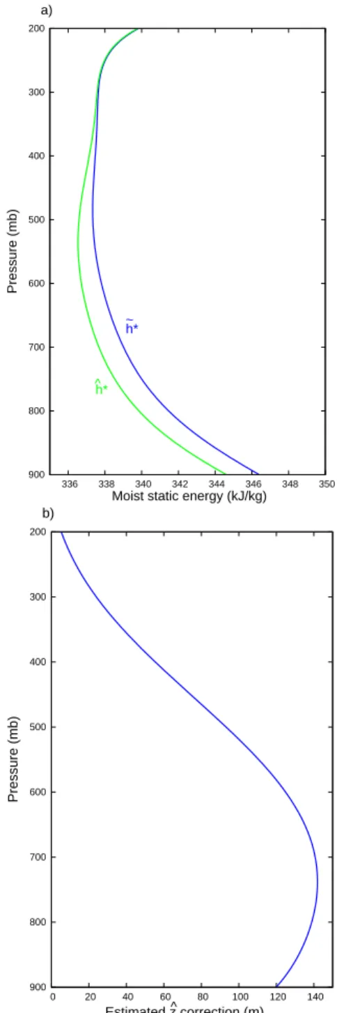
It is straightforward to evaluate the specific-humidity com-ponent ofhvc/eh∗explicitly, and for the Jordan (1958) sound-ing we find that the ratio has a maximum amplitude of around 0.005 in the lower troposphere. Moreover,svc/bsand qvc/bq∗peak at 0.002 and 0.04, respectively, so that it would appear reasonable to neglect virtual effects as being small corrections to in-plume variables in the detrainment layer. However, the purpose of Eq. (11) or (21) is to determinebzi and Fig. 2a shows that the environmental gradient of satu-rated moist static energy is small in the tropical upper tro-posphere. Hence, even small errors in the specification of the neutral-buoyancy condition could result in considerable errors in a calculation of cloud top. Such errors are diffi-cult to estimate reliably when∂eh∗/∂zis small, particularly if there is any noise in theeh∗sounding data. For this reason, in Fig. 2b we plot the quantity

1bz=1

2

svc ∂_es/∂z

+

qvc ∂_eq∗_/∂z

(23) which provides a simple-minded estimate of the effect of vir-tual contributions on the evaluation of cloud top, and which should be reliable for plumes terminating in the lower tropo-sphere. The corrections are∼150 m.

Of course, one could choose to formulate a bulk model with an estimated virtual correction included, leading to Eqs. (11) and (17) but withbl→lB(cf. Nordeng, 1994). This would be an improvement if|lB−bl|<|δ(q∗−q)−bl|

4 Construction of bulk budget

We are now in a position to consider the collective effects of the plume ensemble. In Sect. 4.1 we describe YEC73’s con-struction of a bulk plume, and proceed in Sect. 4.2 to com-pare that to a construction from AS74’s equation set. 4.1 Construction in YEC73

Budget equations for a representative bulk plume are ob-tained in YEC73 by summing over plumes in Eqs. (2) to (5).

0.000 0.005 0.010 0.015 0.020 0.025 0.030 0.035

Massflux (Pa/s)

1000 700

900 800 500

600 300

400 100

200

Pressure (mb)

a)

0.0 0.2 0.4 0.6 0.8 1.0 1.2

Liquid water (g/kg)

1000 900 800 600

700 500 400 100

300 200

Pressure (mb)

b)

Fig. 1. (a) Vertical profiles of mass flux for entraining plumes

launched into the Jordan (1958) sounding. Each plume has an arbi-trary updraft-base mass flux of 0.01 Pas−1and a range of entrain-ment rates are used to produce a range of detrainentrain-ment levels, these being indicated by the diamond symbol. (b) The corresponding pro-files of plume liquid water (blue lines). Also shown are the propro-files of detrained liquid water (red line) and the bulk liquid water for the plume ensemble (green line).

Recalling also points (i) to (iii) from Sect. 2 and the detrain-ment assumptions of Sect. 3.2 then we obtain

E−D−∂M

∂z =0 (24)

E_es−D_es−∂MsB

200

300

400

500

600

700

800

900

336 338 340 342 344 346 348 350

Pressure (mb)

Moist static energy (kJ/kg)

^

h* ~

a)

h*

200

300

400

500

600

700

800

900

0 20 40 60 80 100 120 140

Pressure (mb)

Estimated z correction (m)^ b)

Fig. 2. (a) Vertical profiles ofeh∗ (blue line) andbh∗(green line; Eq. 11) for the Jordan (1958) sounding. (b) Error in the calculation ofbz, as discussed in the main text and estimated from Eq. (23).

E_eq−D_eq −∂MqB

∂z −ρc=0 (26)

−DlB−

∂MlB

∂z +ρc−R=0 (27) where

E=X

i

Ei;D=

X

i

Di;M=

X

i

Mi;R=

X

i

Ri (28)

Other relevant equations for the bulk plume can be ob-tained by taking Eqs. (8) and (9), multiplying byMi, sum-ming over clouds and then dividing byM. This gives sB−s≈

1 1+γ

hB−h ∗

(29)

L(qB−q∗)≈ γ 1+γ

hB−h ∗

(30) The mass-flux approximation for the turbulent flux ofχ (Eq. 7) now reads

ρχ′_w′_{=M (χ}

B−eχ ) (31) There are also two microphysical relations.22 The evapo-ration term is

e=DlB (32)

which is simply obtained from a sum over plumes of23

ei=Dili (33)

The precipitation rate, summed over the full plume ensem-ble, is parameterized as the product oflB with an empirical function of height24

R=k(p)lB (34)

This completes the equation set for the YEC73 bulk model. 4.2 Construction from AS74

The model of YEC73 does not provide a complete descrip-tion of individual entraining plumes. Rather, it posits detrain-ment conditions using bulk quantities, and so Sect. 4.1 does not make plain the relationship between bulk and spectral models. Here we will construct a bulk plume starting from the description of individual plumes in AS74.

Starting from Eqs. (2) to (5), we set the time derivatives to zero and sum over plumes to obtain

E−D−∂M

∂z =0 (35)

Es−X

i

DisDi−∂MsB

∂z +Lρc+ρ

X

i

QRi=0 (36)

Eq−X

i

DiqDi− ∂MqB

∂z −ρc=0 (37)

−X

i

DilDi− ∂MlB

∂z +ρc−R=0 (38) 22_{Equivalent to Eqs. (47) and (48) of YEC73.}

23_{Eq. (31) of YEC73}

24_{Rmust scale with the strength of the convection occurring, and}

so the “empirical function” must be scaled similarly: cf. Eq. (45) for the AS74 formulation. More formally, in the language of Sect. 5,

The next step is to apply the detrainment conditions for

in-dividual plumes from Sect. 3.1. Substituting from Eqs. (14)

to (16) leads to Es−Dbs−∂MsB

∂z +Lρc

e_{=0 (39)}

Eq−Dbq∗− ∂MqB

∂z −ρc

e_{=0 (40)}

−Dbl− ∂MlB

∂z +ρc

e_{−R=0 (41)}

where we have introduced the superscript e to denote a quan-tity which is summed only within the entraining layers of contributing plumes. Shortly we shall also use an analogous superscriptd to denote a quantity summed only within the

detraining layers.

Equations (29) and (30) from the YEC73 bulk system also apply here, as does the mass flux relationship of Eq. (31).

The microphysical equation for evaporation in AS74 is,25 e=X

i ei =

X

i

DilDi (42)

which can be rewritten as

e=Dbl+ρcd (43)

while the rain rate is parameterized as26

Ri =C0Mili (44)

whereC0is a constant. Hence,

R=C0MlB (45)

Clearly the microphysics is extremely simple. Hack et al. (1984) argued that a straightforward improvement would be to setC0differently for deep and shallow clouds.27 But no-tice that ifC0→Ci in Eq. (44) then the simple formula in Eq. (45) can no longer be constructed for a bulk formulation. Rather, some knowledge of the partitioning oflB across the spectrum would be required. Indeed, this is a good example of a general point about the use of more-complicated repre-sentations for individual plumes. In general these will only be well-defined within a spectral formulation, and in essence a bulk formulation is committed to crude microphysics.

Of course, the inclusion of fully realistic microphysics in any mass-flux-based convective parameterization is a diffi-cult issue, since microphysical processes have complex, non-linear dependencies on vertical velocity (e.g. Straka, 2009). Thus, it is no longer sufficient to consider the mass flux alone, but rather the fractional area and vertical velocity must be known separately, which entails carrying an additional equation (e.g Piriou et al., 2007). A spectral formulation is the natural structure for any such attempt, since the averaging inherent in a bulk formulation would not allow one to capture the nonlinearities.

25_{Their Eq. (40)}

26_{See Eqs. (78), (86) and Appendix B (p. 697, statement between}

Eqs. B6 and B7) of AS74.

27_{See their Fig. 3.}

4.3 Comparison of bulk budgets

It may be helpful at this stage to highlight the differences between the two bulk-model equation sets from Sects. 4.1 and 4.2.

1. In the dry-static-energy (Eqs. 25 and 39) and moisture budgets (Eqs. 26 and 40) the differences are:

(a) entrainment ofs (q) for the AS74 model and of_es (_eq) for the YEC73 model.

(b) detrainment of_bs (_bq∗) for the AS74 model and of

es (_eq) for the YEC73 model. This arises because YEC73 neglect virtual effects in the detrainment condition. Note thatbs (bq∗) is a function of both large-scale (overbarred) variables and of the non-bulk, in-plume variablebl(Eqs. 17 and 19). (c) condensation within the detrainment layer is

ex-plicit in the YEC73 model, but imex-plicit in the AS74 model (becausebs6=sDiandbq∗6=qDi).

2. In the liquid-water budgets (Eqs. 27 and 41) the differ-ences are:

(a) detrainment ofblfor the AS74 model and oflB for the YEC73 model.28 Knowledge ofbl(z)requires knowledge of the plume spectrum because for each heightzit has to be determined by integrating the budget equations for an individual plume that de-trains at_bzi=z.

(b) condensation within the detrainment layer is ex-plicit in the YEC73 model, but imex-plicit in the AS74 model (becausebl6=lDi).

3. In the YEC73 model, precipitation is related to an em-pirical function of height, whereas in the AS74 model this function is specified as the product of a constant and the total mass flux (Eqs. 34 and 45).

4. Both models evaporate in-plume water at its detrain-ment level (Eqs. 32 and 43), but the rate is affected by the assumptions on condensation at this level.

5 Normalization transformations

The YEC73 bulk model is designed for diagnostic use and no closure is required. The spectral model of AS74 can also be used in the same way (e.g. Nitta, 1975). However, if a 28_{We do not consider downdrafts here, which are significant in}

bulk or a spectral model is to form the basis of a parameter-ization then it will require closure. Starting from some first guess forM(zbase,λ), the closure is essentially the process of rescaling that guess to obtain the actual amount of convec-tive transport. More formally, the rescaling can be thought of as selecting a privileged member from the set of possible nor-malization transformations. Before proceeding to assess par-ticular closure methods in Sect. 6, it is convenient to define such transformations explicitly and to set out the possible re-sponses of relevant variables.

Normalization transformations,T_{, are applied to the}

spec-tral groupings of Eq. (1). The transformation is a positively-valued rescaling of the updraft-base mass flux for each plume sub-ensemble (or loosely, each cloud type),

M_{(zbase,λ)→}M_(zbase,λ)T_{(λ) (46)}

wherezbasedenotes the updraft base, at the top of the mixed layer. Note that this is distinct from the cloud-base, which we denote aszc(λ), and from the lifting condensation level, zLCL≡zc(0). A subset of normalization transformations of particular interest comprises those for whichT is indepen-dent ofλ, which we will refer to as global transformations.

The importance of normalization transformations arises in considerations of possible timescale separations. A time-evolution operator describing changes in the plume-ensemble between any two times can always be represented as a normalization transformation. We therefore assert that distinct, well-defined responses to a normalization transfor-mation constitute distinct, well-defined timescales character-izing the ensemble.

All of the variables,V, used in this article transform in one of the following ways.

1. Normalization-invariant variables are unaffected by a normalization transformation,V→V∀T_{. Such}

vari-ables may be directly dependent on plume dynamics (e.g.,si), but only through intensive properties of each plume type. They must be independent of the overall amount of convective transport (i.e., ofMandD), and also of its distribution across the plume spectrum (i.e., ofM(zbase,λ)/M(zbase)). They evolve only in response to changes in the large-scale state (i.e., the overbarred variables), which occur on a large-scale timescale of τLS.

2. Globally-invariant variables are unaffected by a global transformation, so thatV→V if and only ifT is inde-pendent of λ. Such variables are independent of the overall amount of convective transport but are sensitive to its distribution across the plume spectrum. Their evo-lution is governed by the timescaleτspec, characterising changes to the spectral distribution under a fixed large-scale condition.

3. Normalization-rescaled variables transform as

V_→V T_(λ)∀T_{. Such variables transform alongside}

one part of the spectrum only, depending extensively on a given plume type λ, but being independent of the rest of the spectrum. They evolve in response to changes in the particular plume type, which can be characterised by a timescale τλ. The timescale must be at least as long as the corresponding plume lifetime because normalization-rescaled terms such as∂ρσi/∂t were filtered out from Eqs. (2)–(5) in Sect. 2.

4. Globally-rescaled variables transform asV→V T if and only ifT is independent ofλ. Such variables depend extensively on the overall amount of convective trans-port and are sensitive to its distribution across the plume spectrum. Their evolution is governed by the timescale τadj introduced by AS74: if all forcing for convection were to be removed then the overall convective trans-port would decay on this timescale.

It may be helpful to clarify the meaning of some of the timescales by considering the limiting case of a step-change in the large-scale forcing, the forcing being held fixed on either side of the step (as in Cohen and Craig, 2004). Mass fluxes associated with specific plume types respond to the step with their specific timescales τλ, but the over-all convective transport, as measured byM(zbase), will ap-proach a new, steady value on the timescaleτadj. However, a more complete adjustment, with the spectral distribution

M(zbase,λ)/M(zbase)also required to approach a new steady state, will require a timescaleτspec. To the best of this au-thor’s knowledge, there is no information available from the literature that would provide good estimates ofτspecand its possible dependencies. However, it would not appear overly difficult to devise idealized CRM simulations with a view to identifying such a timescale.29 We shall show that the timescale is relevant for the closure of bulk mass flux param-eterizations.

6 Closure

To close a parameterization, some additional physical con-straints are imposed which determine the amplitude and spectral distribution of the plume ensemble. As described in Sect. 5 the calculation is performed by rescaling a first guess, and the physical constraints must therefore serve as a gener-ator for the privileged normalization transformation defining the rescaling. For a bulk parameterization, a global trans-formation is sufficient to provide the rescaling, the spectral distribution being implicit in the choice ofE(z).

29_{For a smoothly-varying forcing, adjusted, steady values may}

not be clear. Measures of the lag-correlation between the forcing andM(zbase,λ),M(zbase)andM(zbase,λ)/M(zbase)could then

be used to determine timescalesτλ, τadj and τspec, respectively

In order for a bulk and a spectral model to be capable of providing equivalent parameterizations, there are two neces-sary conditions that we can demand of the closures used:

1. given the generator of a normalization transformation that can be computed for the spectral model, it must be possible to construct from that a generator capable of providing a global transformation that can be computed for the bulk model. Such a global transformation could be used to close the bulk model.

2. the generator of the global transformation that closes the bulk model must respect all the same physical con-straints that were specified in order to formulate the gen-erator for closure of the spectral model.

Below we describe the AS74 spectral-model closure (Sect. 6.1) and then investigate whether it is possible to de-velop an equivalent closure for the corresponding bulk model which meets the conditions above (Sects. 6.2 and 6.3). In Sect. 6.4 we discuss other closure methods in the literature. 6.1 The AS74 closure

The AS74 closure starts from the following equation30 for the kinetic energyK_{of a sub-ensemble of plumes}

∂K(λ)

∂t =A(λ)M(zbase,λ)−D(λ) (47) whereD _{is the dissipation. A is known as the cloud work}

function, and is given by the integrated in-plume buoyancy,31

A(λ)≡

zZD(λ)

zbase

g

cpT

M_(z,λ)

M_(zbase,λ) svp(λ)−sv

dz (48)

HerezDis the detrainment level,sv=cpTv+gz the virtual dry static energy andsvp(λ)its in-plume value. The closure relies on the fact that the time derivative ofAcan be decomposed as,32

dA dt =

dA dt

LS

+ dA

dt

C

≡ ˙ALS+ ˙AC (49)

where the subscripts LS and C refer to “large-scale” and “cloud” contributions, respectively.

It is worth noting that the phrase “large-scale” used by AS74 to describe the forcing of the cloud work function has been criticized (e.g. Randall et al., 1997; Mapes, 1997). In-deed, similar criticisms could be applied to the terminology of “large-scale” as used in studies of cumulus parameteriza-tion more generally. In the absence of a generally-accepted

30_{Eq. (132) of AS74}

31_{Eq. (133) of AS74. More generally, as pointed out by Arakawa}

(1993), analogous closures could be based on any functional of the temperature and moisture profiles that has a threshold describing convective instability.

32_{Eq. (140) of AS74}

and satisfactory alternative, however, we follow the conven-tional, if flawed, terminology here.

With that caveat, we wish to be very clear about the dis-tinction between large-scale and cloud terms. In the language of normalization transformations, the distinction is entirely straightforward. A(λ) is a normalization-invariant, and its time derivative has contributions which are normalization-invariant (theA˙LSpart) and which are globally-rescaled (the

˙

ACpart). Thus, timescalesτLS andτadj are appropriate for

˙

ALSandA˙C, respectively. The physical constraint imposed is the separation of those timescales,τLS≫τadj, which defines the AS74 quasi-equilibrium closure,dA/dt≈0. The closure transformationT_{(λ) can be constructed}33 _{by applying this} constraint to Eq. (49).

6.2 Equivalent AS74 closure for a bulk system? We now consider whether an equivalent AS74 closure can be developed for the corresponding bulk model. Summing over all plumes (or equivalently, integrating over allλ), the kinetic energy equation (Eq. 47) becomes

∂K

∂t =ABM(zbase)−DIS (50) where

K= Z

K_dλ;DIS=

Z

D_{dλ (51)}

AB≡

R

M(zbase,λ)A(λ)dλ

M(zbase)

(52)

=

zTOP Z

zbase

g

cpT M

M(zbase)(svB−sv)dz

We have introducedzTOP=zD(0)to denote the highest de-trainment layer (i.e., that for a non-entraining plume ofλ=0), and have made use of the understanding that there are no con-tributions toM(z)from plumes characterised by aλsuch that z>zD(λ).

The bulk-cloud work functionAB, itself a global invari-ant, has a time derivative that cannot be decomposed into normalization-invariant and globally-rescaled parts. For ex-ample, one contribution to the time derivative is

dAB dt =

Z _M(zbase,λ)

M(zbase)

dA(λ)

dt dλ+ ··· (53)

= R

M(zbase,λ)(A˙LS(λ)+ ˙AC(λ))dλ

M(zbase) + ···

The globally-rescaled variable A˙C produces a globally-rescaled contribution todAB/dt, associated with timescale 33_{In fact, although the constraint can usually be satisfied, it is not}

τadj. The normalization-invariant variableA˙LS(λ), however, does not produce normalization-invariant contributions to dAB/dt. For example,A˙LS(λ)includes a term proportional to changes in mixed-layer moist static-energyhM, and this leads to contributions todAB/dtthat include

dAB dt =

g cpM(zbase)

∂hM ∂t

Z

dλM_{(zbase,λ) (54)}

zZD(λ)

zc(λ)

dz′ 1 T (z′₎

1+γ (z′)ǫ(z′)δ 1+γ (z′₎

+ ···

Although the integral overz′has an integrand that is normal-ization invariant, its limits are functions ofλ. Thus, the con-tribution is globally-invariant, and cannot be evaluated with-out knowledge of the full plume spectrum.

The time-derivative ofABcan in fact be decomposed into globally-invariant and globally-rescaled parts, such that its stationarity could be used to close a bulk parameterization given a constraint that τspec≫τadj. Such a closure would satisfy condition (1) from Sect. 6. It is unclear, however, whetherAB can be considered to be slowly-varying in this sense. Certainly, the imposed AS74 physical constraint of dA(λ)/dt≈0 is no guarantee thatdAB/dt≈0, and so station-arity ofABdoes not satisfy condition (2) for a valid equiva-lent closure of a bulk parameterization.

6.3 CAPE closure of AS74 system?

We have shown that the bulk cloud work function may not be used to close a bulk parameterization in a manner equivalent to the AS74 quasi-equilibrium closure of a spectral param-eterization. However, there may be multiple ways in which a generator to close a spectral parameterization can be re-duced to a generator to close a bulk parameterization. Let us consider the undilute CAPE, or in other words, the cloud work function for a non-entraining plume,

CAPE=A(0)=

zTOP Z

zbase

g

cpT svp(0)−sv

dz (55)

The kinetic energy of non-entraining plumes is described by Eq. (47) and the decomposition ofdA(0)/dt from Eq. (49) applies. Clearly then a CAPE closure usingdA(0)/dt≈0 is physically based uponτLS≫τadj and so would satisfy con-dition (2) for equivalent closure of a bulk parameterization. However, we need to consider also condition (1): whether CAPE closure can act as a generator for a global transforma-tion to allow determinatransforma-tion ofM(zbase).

We examine firstALS(0), the normalization-invariant part˙ ofdA(0)/dt. One of the contributions to this is analogous to the term shown explicitly in Eq. (54) and is specifically

˙

ALS(0)= g

cp ∂hM

∂t zTOP Z

zLCL

dz′ 1 T (z′₎

_{1+γ (z}′_)ǫ(z′_)δ 1+γ (z′₎

+···(56)

The explicit form of terms indA(0)/dt would not normally be used in a parameterization. However, in order for a CAPE-based closure to satisfy condition (1), then it must be possible in principle to evaluate all such terms directly using a bulk model. Examination of all such terms (not shown) reveals that this is indeed the case forA˙LS(0), provided thatzLCLis known by the bulk model. This is required to evaluate the integral in Eq. (56) for instance. In Appendix A we demon-strate that under normal conditionszc≥zLCL, and sozLCLis simply the lowest height for whichlB6=0. This inequality is important and explains why it is necessary to use CAPE: it would not be valid according to condition (1) to try to close a bulk parameterization using the cloud work function for any non-zero value ofλ.

Consider now AC(0), the globally-rescaled part of˙ dA(0)/dt. This can be categorized into mixed-layer terms, vertical mass-flux terms and detrainment terms.34 The mixed-layer terms can be evaluated from the environmen-tal sounding and the toenvironmen-tal updraft-base mass fluxM(zbase), while the vertical mass-flux terms require knowledge of the full functionM(z). The detrainment terms include the fol-lowing contribution

˙

AC(0)= gL

cp zZTOP

zLCL

dz 1

ρTD(z)[1−(1+δ)ǫ]bl+ ··· (57) This requires the detrainment profileD(z)and the quantity

bl. The latter is problematic for a bulk parameterization, be-cause it should properly be computed by integrating the bud-get equations for a single plume (Sect. 3.1). Thus, the sta-tionarity of CAPE does not satisfy condition (1) for a valid equivalent closure of a bulk parameterization.35 _The prob-lem can be avoided by invoking again the ansatz of Eq. (20) that was introduced in Sect. 3.2 in order to formulate detrain-ment in the bulk-plume budget equations. We have shown then that the ansatz is required not only to compute the ver-tical profile of the bulk plume but that it is also necessary to permit CAPE closure36of a bulk parameterization. The prac-tical impact of the ansatz on closure calculations is difficult to discern: certainly this author is unaware of any attempt in the literature to assess the impact.

34_{See Eqs. (141), (144) and (B35) of AS74.}

35_{In a re-derivation of the AS74 model by the present author,}

some additional terms inA˙C(0)were obtained that do not appear in

AS74. These are proportional to the microphysical quantityd(z,λ)

defined by Eq. (B20) of AS74, and one such term also involvesbl. However, none of these terms affect any of the arguments presented on the formal validity of CAPE closure.

36_{Instead of using a cloud work function, some recent authors}

(e.g Kain et al., 2003; Kain, 2004; Zhang, 2009) have investi-gated the use of dilute CAPE for the closure of bulk parameteri-zation. Dilute CAPE differs from CAPE by substitutingsvB for

svp(0)in Eq. 55, or equivalently, fromAB by omitting the factor

6.4 Other closures

We have considered in some detail the AS74 quasi-equilibrium closure for spectral models of entraining plumes. However, many other closures have been proposed for con-vective parameterizations, at least in part because any given closure may appear more or less plausible over different lo-cations and with different grid-box sizes in the parent model (e.g. Grell et al., 1991; Grell, 1993). It would neither be prac-tical nor instructive to consider every one, but some remarks on how other types of closure might apply to bulk and spec-tral parameterizations would seem to be in order.

Various authors have suggested various classifications of closure assumptions, but Grell et al.’s (1991, p. 6) is the most appropriate for our present purposes.37 Closures seek to re-late the overall convective transport to: (i) a measure of large-scale instability, by imposing an adjustment of that mea-sure; (ii) a measure of large-scale advection, typically hor-izontal mass or moisture convergence; or, (iii) a measure of the rate of environmental destabilization. The AS74 closure is of class (iii), constraining the generation of a vertically-integrated instability measure. Other closures with a simi-lar basis (e.g. Moorthi and Suarez, 1992; Pan and Randall, 1998; Byun and Hong, 2007) will also have formal difficul-ties if applied to a bulk parameterization. The key point of difficulty for bulk models is the detrainment of condensate, and this will enter into considerations of the rate of change of environmental instability if a vertically-integrated measure encompasses the detrainment layer of any plume within the ensemble.

Closures in class (i) are popular particularly in mesoscale models and for mid-latitude applications (e.g. Frank, 1983). Typically, such a closure aims to remove CAPE, sometimes instantaneously upon convective triggering but more com-monly within some “closure timescale”, which is just theτadj of Sect. 5 (e.g. Fritsch and Chappell, 1980; Emanuel, 1993; Zhang and McFarlane, 1995; Gregory, 1997; Willett and Mil-ton, 2006; Bechtold et al., 2001; Kain, 2004). This method is inspired by observations in which the triggering of a convec-tive episode does indeed consume preexisting instability (e.g. Fritsch et al., 1976; Song and Frank, 1983). The removal is described by Eq. (49) forλ=0, and therefore the issue raised in Sect. 6.3 also applies to such closures. For a bulk parame-terization, the removal of CAPE is not a well-defined closure unless one invokes the YEC73 ansatz.

Conceptually, the closures in class (ii) (e.g. Kuo, 1974; Tiedtke, 1989; Frank and Cohen, 1987; Brown, 1979) use empirical relationships betweenM(zbase)and various mea-sures of large-scale advection. Thus, they generate global 37_{It is not always entirely clear that a particular closure belongs}

uniquely to a particular class. For example, McBride (1981) showed that the AS74 closure is actually strongly dependent on horizontal mass convergence, and its vertical distribution. See also Arakawa (2004). Nonetheless, the classification is adequate for our discus-sion.

transformations that can in principle be applied freely to bulk and spectral parameterizations alike. Not seeking to revisit such debates here, we simply note that closures from this class have become markedly less popular over recent years, not least as a result of attacks on their conceptual basis from Emanuel (1994); Raymond and Emanuel (1993); Arakawa (2004) and others.

Our discussion has focussed on the formal validity (or oth-erwise) of the generators of global transformations for bulk parameterizations. It is important, however, that the reader should not be left with an impression that closure of a spec-tral parameterization is a simple matter. A physical con-straint that can act as a global transformation generator is sufficient to close a bulk parameterization, but would provide none of the necessary information to a spectral parameteriza-tion about the spectral distribuparameteriza-tion of mass flux. Some spec-tral parameterizations apply constraints to generate explic-itly a suitable normalization transformation (Arakawa and Schubert, 1974; Nober and Graf, 2005), while others com-bine instead a global transformation with some additional constraints to set the spectral distribution, whether by appeal to observations (e.g. Donner, 1993), or theory (e.g. Plant and Craig, 2008), or even “mainly for the sake of simplicity” (e.g. Zhang and McFarlane, 1995, p. 412). Regardless of the ap-proach taken, setting the spectral distribution is not trivial.

7 Conclusions

Key aspects of climate models, for example the moisture structure in the tropics (e.g. Gregory, 1997), are highly sen-sitive to the formulation of entrainment in the convection pa-rameterization (e.g. Knight et al., 2007). In a spectral model of plumes simple treatments are generally used for the en-trainment into a single plume, but these become translated into overallE(z)andD(z)that are complicated functions of the environment. Such functions would be difficult to specify directly, and AS74 claim in effect that this makes a spectral formulation the natural choice. In a bulk model,E(z) and D(z)are chosen by the modeller,38often with some switch-ing of the functional forms between “types” (e.g. Gregory, 1997) according to the large-scale regime. Thus, a bulk pa-rameterization offers the modeller more direct control over its behaviour. Whether this is considered to be a good or a bad point is to some extent an issue of the modelling philos-ophy.

38_{Relatively sophisticated treatments of entrainment and}

The differences between bulk and spectral parameteriza-tions are perhaps most often thought about in terms of the specification of entrainment and detrainment, but there are also differences in the underlying theoretical structure. The theoretical differences have been the subject of this article. Budget equations for individual and for bulk plumes can be cast into very similar forms (Sect. 4) provided that an ansatz is made for the detrainment of condensate from the bulk plume. The ansatz is thatlDi=lB (Eq. 20) and is the price paid for the simplification to a single bulk plume. Moreover, similarity between the equation sets requires a very simple representation of the microphysics. The use of more com-plicated microphysics in bulk convective parameterizations lacks a sound theoretical basis.

While Yanai et al. (1973) are clear about the arbitrary, but convenient, nature of their ansatz, that is not always the case in later works. For example, one issue for convective param-eterization is the coupling to stratiform cloud. Motivated by considerations of mesoscale organization, some authors (e.g. Frank and Cohen, 1987; Kain, 2004; Kreitzberg and Perkey, 1976) have taken a so-called “hybrid approach” (Molinari and Dudek, 1992), in which (a fraction of) the detrained con-densate is acted upon by the parent model’s large-scale cloud equations, allowing it to act as a source term for prognostic respresentations of stratiform cloud (e.g. Fowler et al., 1996; Tiedtke, 1993). Such treatments can have significant effects: for example, on cirrus and on the hydrological cycle in the tropics (e.g. Tiedtke, 1993; Liu et al., 2001). In the opinion of this author, however, much of the relevant literature does not seem to appreciate fully, or sometimes even to recognize, Yanai et al.’s (1973) ansatz: while the detrained condensate is predicted by a spectral parameterization, the values ob-tained from a bulk parameterization are systematic overesti-mates that by construction are not intended to be reliable.

Another consequence of Yanai et al.’s (1973) ansatz is that virtual temperature effects must be approximated or even ig-nored in determining the bulk plume top (Sect. 3). Moreover, there is not necessarily an equivalence between closure con-straints applied to spectral and bulk parameterizations.

Closures based on CAPE, or a cloud-work function, as-sume a timescale separation between the slow mechanisms of atmospheric destablization and the relatively fast mech-anisms of the convective response. The definition and in-terpretation of the slow and fast timescales has been much debated. In Sect. 5 we introduced a normalization transfor-mation, and argued that the behaviour of a variable under such a transformation is sufficient to associate that variable with a well-defined timescale. We were then able to show that the quasi-equilibrium closure for spectral parameteriza-tions introduced by Arakawa and Schubert (1974) does not correspond in any straightforward way to a suitable closure constraint for bulk parameterizations. The natural analogue to the Arakawa and Schubert (1974) closure is the stationar-ity of the bulk cloud work function, but the evolution of this variable is governed by timescalesτspecandτadj(Sect. 6.2),

rather than the timescales τLS andτadj governing the evo-lution of the cloud work function A(λ)(Sect. 6.1). Thus, the stationarity ofAB andA(λ)would encapsulate distinct physical constraints. τspecandτLSdo not seem to have been clearly distinguished before now, let alone studied in any sys-tematic way.

This timescale issue can be avoided if one closes a bulk parameterization using either the removal of CAPE by the plume ensemble or a quasi-equilibrium constraint of dCAPE/dt≈0. It should be noted, however, that a computa-tion ofdCAPE/dt involves the detraining condensate from each plume, and so cannot be performed by a bulk model, un-less the Yanai et al. (1973) ansatz is used. Thus, the ansatz is a necessary ingredient in such a closure (Sect. 6.3). Whether this has a practical impact on the closure of bulk parameteri-zations has not been examined in the literature.

In comparing a “full” and a “simplified” physical model, there is always a danger of confusing complexity with so-phistication. Most convective parameterizations in use today are of the bulk form, and this is undoubtedly a convenient simplification that should not be discarded lightly. It is ob-tained by invoking Yanai et al.’s (1973) ansatz and has im-plications for: the microphysics of convective and associated layer cloud; the calculation of cloud top; and, the validity of closure methods for bulk parameterization. Some of those implications were previously known, but perhaps obscure, whereas others have been raised here. The extent to which such theoretical issues with the structure of bulk parameter-izations may affect their actual performance in practice is not well studied, but systematic investigations are required if modellers are to make well-informed judgements about the continued use of bulk parameterizations. The question to be continually asked is not so much is a bulk or a

spec-tral method to be preferred? but rather is the bulk framework conceptually “good enough” for our present and future pur-poses?.

Appendix A Cloud base level

The purpose of this Appendix is to demonstate that under normal atmospheric conditions then zc≥zLCL, as stated in Sect. 6.3: i.e., that cloud base for an entraining plume lies above that for a non-entraining plume.

Cloud base is defined in AS74 to be the lowest height at which Eq. (8) is satisfied, describing the saturation of in-plume air. It is convenient to restate that equation here,

sp−s≈ 1 1+γ

hp−h ∗

forz≥zc(λ) (A1)

ini-tial conditions39 taken from the mixed-layer properties, sp(zbase)=sMandhp(zbase)=hM. For a non-entraining plume spandhpretain their initial values and sozLCLis defined by the lowest height which satisfies

sM−s≈ 1 1+γ

hM−h ∗

forz≥zLCL (A2)

Now, given two equationsg1(z1)=0 andg2(z2)=0 then if g2≈g1, a simple Taylor series expansion ofg2aboutz1yields

z1−z2=

g2(z1)−g1(z1) g′

2(z1)

(A3)

the dash here denoting a vertical derivative. Applying this to the above equations defining cloud base, we have

zc−zLCL=

γ (sp−sM)−L(qp−qM)

gγ +sγ′

zc

(A4)

where we have used the definitions ofγ ands to simplify the denominator. For water vapour bothγ andγ′are posi-tive, and so the denominator must be positive. Thus, if the numerator is also positive, thenzc≥zLCLas required.

Consider the two bracketed terms in the numerator. As-suming thatsincreases monotonically with height between zbase andzc (i.e., that the lapse rate is no stronger than dry adiabatic), then the entrainment process must produce values ofspthat are larger thansM. Similarly a monotonic decrease ofqwithin the environment must produceqp(zc)<qM. Un-der normal atmospheric conditions therefore, the numerator is indeed positive.

Appendix B

Nomenclature: Symbols not explicitly listed below have their standard meteorological meanings.

χvc subscript denoting a virtual contribution χB subscript denoting a bulk value

χi subscript denoting a specific plume χC subscript denoting a cloud term χLS subscript denoting a large-scale term χM subscript denoting a mixed-layer value χp subscript denoting an in-plume value

χDi subscript denoting value on detrainment from plumei

χ′ prime denoting deviation from horizontal mean χ∗ superscript denoting saturated value

χd superscript denoting a quantity to be evaluated in the detraining layers of contributing plumes only

39_{Eqs. (129) and (131) of AS74}

χe superscript denoting a quantity to be evaluated in the entraining layers of contributing plumes only

˙

χ time derivative ofχ

χ horizontally-averaged value ofχ

b

χ value at the detrainment level

e

χ environmental value ofχ

δ thermodynamic parameter: one less than the ra-tio of gas constants of water vapour to dry air ǫ thermodynamic parameter defined by Eq. (13) γ thermodynamic parameter defined by Eq. (10) λ parameter defining an entraining plume type σ fractional area covered by plume

τλ timescale for plume typeλ

τadj adjustment timescale for overall amplitude of convective activity

τLS large-scale timescale

τspec timescale for changes to spectral distribution under a fixed large-scale condition

D _{rate of kinetic energy dissipation} K _{kinetic energy}

T _{normalization transformation}

A cloud work function c rate of condensation

C0 constant defining the autoconversion rate in the system of AS74, via Eq. (44)

D detrainment rate E entrainment rate e evaporation rate h moist static energy

K total kinetic energy of plume ensemble

k empirical function defining the autoconversion rate in the system of YEC73, via Eq. (34) l plume liquid water

M convective mass flux QR radiative heating rate R conversion rate s dry static energy sv virtual dry static energy

svp in-plume value of virtual dry static energy zbase base level for entraining plumes

zLCL lifting condensation level

zTOP highest detrainment level from the plume en-semble

zD detrainment level zc cloud base level

DIS total dissipation rate of plume ensemble

Acknowledgements. A conversation with P. Siebesma and

J.-I. Yano at the Workshop on Concepts for Convective Parameteri-zations in Large-Scale Models first inspired me to delve into these issues.

References

Arakawa, A.: Closure assumptions in the cumulus parameterization problem, in: The Representation of Cumulus Convection in Nu-merical Models, edited by: Emanuel, K. A. and Raymond, D. J., of Meteorological Monographs, chap. 1, Am. Meteorol. Soc., 24, 1–16, 1993.

Arakawa, A.: The cumulus parameterization problem: past, present and future, J. Climate, 17, 2493–2525, 2004.

Arakawa, A. and Schubert, W. H.: Interaction of a cumulus cloud ensemble with the large-scale environment, Part I, J. Atmos. Sci., 31, 674–701, 1974.

Bechtold, P., Bazile, E., Guichard, F., and Richard, E.: A mass-flux convection scheme for regional and global models, Q. J. Roy. Meteor. Soc., 127, 869–886, 2001.

Betts, A. K. and Miller, M. J.: A new convective adjustment scheme, Part II: single column tests using GATE wave, BOMEX, ATEX and arctic air-mass data sets, Q. J. Roy. Meteor. Soc., 112, 793–809, 1986.

Bougeault, P.: A simple parameterization of the large-scale effects of cumulus convection, Mon. Weather Rev., 113, 2108–2121, 1985.

Brown, J. M.: Mesoscale unsaturated downdrafts driven by rain-fall evaporation: a numerical study, J. Atmos. Sci., 36, 313–338, 1979.

Byun, Y.-H. and Hong, S.-Y.: Improvements in the subgrid-scale representation of moist convection in a cumulus parameteriza-tion scheme: the single-column test and its impact on seasonal prediction, Mon. Weather Rev., 135, 2135–2154, 2007. Cho, H.-R.: Contributions of cumulus cloud life-cycle effects to the

large-scale heat and moisture budget equations, J. Atmos. Sci., 34, 87–97, 1977.

Cohen, B. G. and Craig, G. C.: The response time of a convective cloud ensemble to a change in forcing, Q. J. Roy. Meteor. Soc., 130, 933–944, 2004.

Donner, L. J.: A cumulus parameterization including mass fluxes, vertical momentum dynamics, and mesoscale effects, J. Atmos. Sci., 50, 889–906, 1993.

Emanuel, K. A.: A cumulus representation based on the episodic mixing model: the importance of mixing and microphysics in predicting humidity, in: The Representation of Cumulus Con-vection in Numerical Models, edited by: Emanuel, K. A. and Raymond, D. J. of Meteorological Monographs, Am. Meteorol. Soc., 19(24), 185–192, 1993.

Emanuel, K. A.: Atmospheric Convection, Oxford University Press, 1994.

Esbensen, S.: Bulk thermodynamic effects and properties of small tropical cumuli, J. Atmos. Sci., 35, 826–837, 1978.

Fowler, L. D., Randall, D. A., and Rutledge, S. A.: Liquid and ice cloud microphysics in the CSU general circulation model, Part 1: model description and simulated microphysical processes, J. Cli-mate, 9, 489–529, 1996.

Frank, W. M.: The cumulus parameterization problem, Mon. Weather Rev., 111, 1859–1871, 1983.

Frank, W. M. and Cohen, C.: Simulation of tropical convective systems, Part I: a cumulus parameterization, J. Atmos. Sci., 44, 3787–3799, 1987.

Fritsch, J. M. and Chappell, C. F.: Numerical prediction of con-vectively driven mesoscale pressure systems, Part I: convective parameterization, J. Atmos. Sci., 37, 1722–1733, 1980.

Fritsch, J. M. and Kain, J. S.: Convective parameterization for mesoscale models: the Fritsch-Chappell scheme, in: The Rep-resentation of Cumulus Convection in Numerical Models, edited by: Emanuel, K. A. and Raymond, D. J. of Meteorological Monographs, Am. Meteorol. Soc., 24(15), 159–164, 1993. Fritsch, J. M., Chappell, C. F., and Hoxit, L. R.: The use of

large-scale budgets for convective parameterization, Mon. Weather Rev., 104, 1408–1418, 1976.

Garner, S. T., Frierson, D. M. W., Held, I. M., Pauluius, O., and Vallis, G. K.: Resolving convection in a global hypohydrostatic model, J. Atmos. Sci., 64, 2061–2075, 2007.

Gerard, L. and Geleyn, J.-F.: Evolution of a subgrid deep convection parameterization in a limited-area model with increasing resolu-tion, Q. J. Roy. Meteorol. Soc., 131, 2293–2312, 2005.

Gregory, D.: The mass flux approach to the parameterization of deep convection, in: The Physics and Parameterization of Moist Atmospheric Convection, edited by: Smith, R. K., Kluwer Aca-demic Publishers, 297–319, 1997.

Gregory, D. and Rowntree, P. R.: A mass flux convection scheme with representation of cloud ensemble characteristics and stability-dependent closure, Mon. Weather Rev., 118, 1483– 1506, 1990.

Grell, G. A.: Prognostic evaluation of assumptions used by cumulus parameterizations, Mon. Weather Rev., 121, 764–787, 1993. Grell, G. A., Kuo, Y.-H., and Pasch, R. J.: Semiprognostic tests of

cumulus parameterization schemes in the middle latitudes, Mon. Weather Rev., 119, 5–31, 1991.

Hack, J. J., Schubert, W. H., and Dias, P. L. S.: A spectral cumu-lus parameterization for use in numerical models of the tropical atmosphere, Mon. Weather Rev., 112, 704–716, 1984.

Johnson, R. H.: The role of convective-scale precipitation down-drafts in cumulus and synoptic-scale interactions, J. Atmos. Sci., 33, 1890–1910, 1976.

Johnson, R. H.: The effects of cloud detrainment on the diagnosed properties of cumulus populations, J. Atmos. Sci., 34, 359–366, 1977.

Johnson, R. H. and Young, G. S.: Heat and moisture budgets of tropical mesoscale anvil clouds, J. Atmos. Sci., 40, 2138–2147, 1983.

Jordan, C. L.: Mean soundings for the West Indies area, J. Meteo-rol., 15, 91–97, 1958.

Kain, J. S.: The Kain-Fritsch convective parameterization: an up-date, J. Appl. Meteorol., 43, 170–181, 2004.

Kain, J. S. and Fritsch, J. M.: A one-dimensional entrain-ing/detraining plume model and its application in convective pa-rameterization, J. Atmos. Sci., 47, 2784–2802, 1990.

Kain, J. S., Fritsch, J. M., and Weiss, S. J.: Parameterized updraft mass flux as a predictor of convective intensity, Weather Fore-cast., 18, 106–116, 2003.

Khairoutdinov, M., Randall, D., and DeMott, C.: Simulations of the atmospheric general circulation using a cloud-resolving model as a superparameterization of physical processes, J. Atmos. Sci., 62, 2136–2154, 2005.

Kreitzberg, C. W. and Perkey, D. J.: Release of potential instability: Part I. A sequential plume model within a hydrostatic primitive equation model, J. Atmos. Sci., 33, 456–475, 1976.

Kuang, Z. and Bretherton, C. S.: A mass-flux scheme view of a high-resolution simulation of a transition from shallow to deep convection, J. Atmos. Sci., 63, 1895–1909, 2006.

Kuo, H.-L.: Further studies of the parameterization of the influence of cumulus convection on large-scale flow, J. Atmos. Sci., 31, 1232–1240, 1974.

Lawrence, M. G. and Rasch, P. J.: Tracer transport in deep con-vective updrafts: plume ensemble versus bulk formulations, J. Atmos. Sci., 62, 2880–2894, 2005.

Lin, C.: Some bulk properties of cumulus ensembles simulated by a cloud-resolving model, Part II: entrainment profiles, J. Atmos. Sci., 56, 3736–3748, 1999.

Lin, C. and Arakawa, A.: The macroscopic entrainment processes of simulated cumulus ensemble, Part II: testing the entraining-plume model, J. Atmos. Sci., 54, 1044–1053, 1997.

Liu, C., Moncrieff, M. W., and Grabowski, W. W.: Explicit and parameterized realizations of convective cloud systems in TOGA COARE, Mon. Weather Rev., 121, 1689–1703, 2001. Lord, S. J. and Arakawa, A.: Interaction of a cumulus cloud

ensem-ble with the large-scale environment, Part III: semi-prognostic tests of the Arakawa–Schubert cumulus parameterization, J. At-mos. Sci., 39, 88–103, 1982.

Lord, S. J., Chao, W. C., and Arakawa, A.: Interaction of a cumulus cloud ensemble with the large-scale environment, Part IV: the discrete model, J. Atmos. Sci., 39, 104–113, 1982.

Mapes, B. E.: Equilibrium vs. activation control of large-scale vari-ations of tropical deep convection, in: The Physics and Param-eterization of Moist Atmospheric Convection, edited by: Smith, R. K., Kluwer Academic Publishers, 321–358, 1997.

McBride, J. L.: An analysis of diagnostic cloud mass flux models, J. Atmos. Sci., 38, 1977–1990, 1981.

Molinari, J. and Dudek, M.: Parameterization of convective precip-itation in mesoscale numerical models: a critical review, Mon. Weather Rev., 120, 326–344, 1992.

Moorthi, S. and Suarez, M. J.: Relaxed Arakawa-Schubert: a pa-rameterization of moist convection for general circulation mod-els, Mon. Weather Rev., 120, 978–1002, 1992.

Nitta, T.: Observational determination of cloud mass flux distribu-tions, J. Atmos. Sci., 32, 73–91, 1975.

Nitta, T.: Response of cumulus updraft and downdraft to GATE A/B-scale motion systems, J. Atmos. Sci., 34, 1163–1186, 1977.

Nober, F. J. and Graf, H. F.: A new convective cloud

field model based on principles of self-organisation, Atmos. Chem. Phys., 5, 2749–2759, 2005, http://www.atmos-chem-phys.net/5/2749/2005/.

Nordeng, T. E.: Extended versions of the convective parameteri-zation scheme at ECMWF and their impact on the mean and transient activity of the model in the tropics, Technical Memo-randum 206, ECMWF, 1994.

Pan, D.-M. and Randall, D. A.: A cumulus parameterization with prognostic closure, Q. J. Roy. Meteor. Soc., 124, 949–981, 1998. Plant, R. S. and Craig, G. C.: A shocastic parameterization for deep convection based on equilibrium statistics, J. Atmos. Sci., 65, 87–105, 2008.

Piriou, J. M., Redelsperger, J.-L., Geleyn, J.-F., Lafore, J.-P., and Guichard, F.: An approach for convective parameterization with

memory: Separating microphysics and transport in grid-scale equations, J. Atmos. Sci., 64, 4127–4139, 2007.

Randall, D. A., Pan, D.-M., Ding, P., and Cripe, D. G.: Quasi-Equilibrium, in: The Physics and Parameterization of Moist At-mospheric Convection, edited by: Smith, R. K., Kluwer Aca-demic Publishers, 359–385, 1997.

Randall, D. A., Wood, R. A., Bony, S., Colman, R., Fichefet, T., Fyfe, J., Kattsov, V., Pitman, A., Shukla, J., Srinivasan, J., Stouf-fer, R. J., Sumi, A., and Taylor, K. E.: Climate models and their evaluation, in: Climate Change 2007: The Physical Basis, Con-tribution of Working Group I to the Fourth Assessment Report of the Intergovernmental Panel on Climate Change, edited by: Solomon, S., Qin, D., Manning, M., Chen, Z., Marquis, M., Av-eryt, K. B., Tignor, M., and Miller, H. L., Cambridge University Press, Cambridge, UK and New York, NY, USA, 2007. Raymond, D. J. and Blyth, A. M.: A stochastic mixing model for

nonprecipitating cumulus clouds, J. Atmos. Sci., 43, 2708–2718, 1986.

Raymond, D. J. and Emanuel, K. A.: The Kuo cumulus parameter-ization, in: The Representation of Cumulus Convection in Nu-merical Models, edited by: Emanuel, K. A. and Raymond, D. J. of Meteorological Monographs, Am. Meteorol. Soc., 24(10), 145–147, 1993.

Shutts, G. and Allen, T.: Sub-gridscale parametrization from the perspective of a computer games animator, Atmos. Sci. Lett., 8, 85–92, 2007.

Song, J.-L. and Frank, W. M.: Relationship between deep convec-tion and large-scale processes during GATE, Mon. Weather Rev., 111, 2145–2160, 1983.

Straka, J. M.: Cloud and Precipitation Microphysics: Principles and Parameterizations, Cambridge University Press, 2009.

Swann, H.: Evaluation of the mass-flux approach to parametrizing deep convection, Q. J. Roy. Meteor. Soc., 127, 1239–1260, 2001. Tiedtke, M.: A comprehensive mass flux scheme for cumulus pa-rameterization in large-scale models, Mon. Weather Rev., 117, 1779–1800, 1989.

Tiedtke, M.: Representation of clouds in large-scale models, Mon. Weather Rev., 121, 3040–3061, 1993.

Willett, M. R. and Milton, S. F.: The tropical behaviour of the con-vective parameterization in aquaplanet simulations and the sen-sitivity to timestep, Forecasting Research Technical Report 482, Met Office, UK, 2006.

Xu, K.-M. and Randall, D. A.: Influence of large-scale advective colling and moistening effects on the quasi-equilibrium behavior of explicitly simulated cumulus ensembles, J. Atmos. Sci., 55, 896–909, 1998.

Yanai, M. and Johnson, R. H.: Impacts of cumulus convection on thermodynamic fields, in: The Representation of Cumulus Con-vection in Numerical Models, edited by: Emanuel, K. A. and Raymond, D. J. of Meteorological Monographs, Am. Meteorol. Soc., 24(4), 39–62, 1993.

Yanai, M., Esbensen, S., and Chu, J.-H.: Determination of bulk properties of tropical cloud clusters from large-scale heat and moisture budgets, J. Atmos. Sci., 30, 611–627, 1973.

Yanai, M., Chu, J.-H., Starx, T. E., and Nitta, T.: Response of deep and shallow tropical maritime cumuli to large-scale processes, J. Atmos. Sci., 33, 976–991, 1976.

Roy. Meteor. Soc., 126, 1861–1887, 2000.

Yano, J.-I., Guichard, F., Lafore, J.-P., Redelsperger, J.-L., and Bechtold, P.: Estimations of mass fluxes for cumulus parame-terizations from high-resolution spatial data, J. Atmos. Sci., 61, 829–842, 2004.

Zhang, G. J. and McFarlane, N. A.: Sensitivity of climate simula-tions to the parameterization of cumulus convection in the Cana-dian climate centre general circulation model, Atmos.-Ocean, 33, 407–446, 1995.