Measuring the complex behavior of the SO2 oxidation reaction

(1)

Article

Measuring the complex behavior of the SO

2

oxidation reaction

Muhammad Shahzad1, Sumaira Rehman1, Rabia Bibi1, Hafiz Abdul Wahab1, Saleem Abdullah1,

Sarfraz Ahmed2 1

Department of Mathematics, HazaraUniversity, Mansehra, 21300, Pakistan 2

Department of Mathematics, Abbottabad University of Science and Technology, Abbottabad, Pakistan E-mail: shahzadmaths@hu.edu.pk

Received 27 April 2015; Accepted 5 June 2015; Published 1 September 2015

Abstract

The two step reversible chemical reaction involving five chemical species is investigated. The quasi equilibrium manifold (QEM) and spectral quasi equilibrium manifold (SQEM) are used for initial approximation to simplify the mechanisms, which we want to utilize in order to investigate the behavior of the desired species. They show a meaningful picture, but for maximum clarity, the investigation method of invariant grid (MIG) is employed. These methods simplify the complex chemical kinetics and deduce low dimensional manifold (LDM) from the high dimensional mechanism. The coverage of the species near equilibrium point is investigated and then we shall discuss moving along the equilibrium of ODEs. The steady state behavior is observed and the Lyapunov function is utilized to study the stability of ODEs. Graphical results are used to describe the physical aspects of measurements.

Keywords chemical kinetics; key variables; slow manifold; refinement; Lyapunov function.

1 Introduction

Chemical materials play an effective role, not only in our daily life, such as plastics and different types of drinks, but they are also used for manufacturing defense equipments. The chemical industry is a necessary part of our development as it deals with diverse chemical reactions such as catalytic reactions, which have numerous applications in chemical industries including newly emerging applications in fine chemicals and pharmaceuticals (Roy and Chaudhari, 2005). So, the analysis of such chemical reactions has great importance. These chemical reactions vary from simple to complex depending on their corresponding nature. Gas-solid catalytic reactions are complex reactions taking place in industrial chemical processes. So it needs their theoretical and experimental investigations. Different approaches and methods have been developed for analyzing different aspects of linear chemical reactions by several researchers (Gorban and Karlin, 2003; Hangos, 2010; Roy and Chaudhari, 2005). On the other hand, due to the complexity of nonlinear chemical reactions, less attention is given to their studies. In this paper, an attempt is made to reduce the complexity and explore hidden aspects of some nonlinear chemical reactions (either fast or slow).

Computational Ecology and Software ISSN 2220721X

URL: http://www.iaees.org/publications/journals/ces/onlineversion.asp RSS: http://www.iaees.org/publications/journals/ces/rss.xml

Email: ces@iaees.org EditorinChief: WenJun Zhang

(2)

Computational Ecology and Software, 2015, 5(3): 254-270

IAEES www.iaees.org 2 Paper Organization

Most chemical reactions have two steps in terms of the rate of occurrence i.e. fast processes and slow processes. The fast processes relax much faster than slower ones. During the relaxation, trajectories in the phase space move towards lower dimensions and converge towards the equilibrium point and after that, they start moving along it (Chiavazzo et al., 2007). This concept is represented with the help of LDM in section 2 where the system is reduced into two species in sub-section 2.2. While the steady state behavior (Bothe and Pierre, 2010; Segel and Slemrod, 1989) of the species also approaches towards the equilibrium point after completing the transition period (Fig. 3), the flow of a vector field near the equilibrium is combined with the initial approximate solution of QEM (Fig. 5).

The general idea of grid construction is given in section 3 to measure a one/higher dimension manifold. While for stability measure we use Lyapunov function is described in section 3.1.

As the solution given by QEM (Fig. 2) is far away from the exact solution shown in section 4, it is refined with the MIG (Fig. 4a, 4b). The other way left is to apply a more accurate method, for which, we apply the SQEM method (Fig. 6a) because it gives a better approximation than QEM. This is then proved by applying MIG over it and no change in the approximated 1D solution is observed (Fig. 6b). Therefore, we proceed towards the two dimensional manifold by applying the concept of SQEM and measure the 2D surface (Fig. 7). The variation in eigen values during the whole process, which is given by fast and slow processes, is calculated (Fig. 8). Finally, we conclude results in section 5.

3 Background

Different chemical reactions have different structural natures as well as distinct kinetic behaviors depending on the type of species. As a consequence of the diverse nature of chemical kinetic structures, corresponding equations can be associated with several time scales. Many physical aspects of chemical reactions are described by Slow Manifold (SM) in a better way. Thus SM plays a key role in the analysis of kinetics in chemical reactions of associated species. There are various approaches, (Chiavazzo and Karlin, 2008; Maas and Pope, 1992b; Muhammad Shahzad, 2015; Succi, 2006) which eliminate fast variables and reduce corresponding equations of the considered system into Slow Manifold (SM). Few of them are recently introduced and they are discussed in this paper in detail.

Slow Invariant Manifold (SIM) provides a simple way to study the dissipative systems of chemical kinetics and the computation of SIM after reducing the system in lower dimensions does not affect the accuracy of results.

4 Experiments

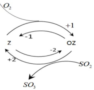
Fig a. General example of two steps, reversible reaction involving five chemical species. In the first step, 2

O react with Z (catalyst) and transformed into Z-oxide. Second step, OZ oxidizes sulphur dioxide into sulphur tri-oxide and re obtain Z. While +, - are the forward and backward reactions and 1, 2 indicates first and second step reactions.

(3)

1 1

2 2

1 2

0.5

2 3

2 k 2

k k

k

O Z OZ

OZ SO SO Z













 

 

(a)

2 1

,

2

,

3

,

2 4

,

3 5

O



c Z



c OZ



c SO



c

SO



c

1

0.5,

2

0.1,

3

0.1,

4

0.4,

5

0.1

eq eq eq eq eq

c



c



c



c



c



In this two-step heterogeneous nonlinear

SO

₂ oxidation reaction, five chemical components

2 2 3

(

O Z OZ SO SO

, ,

,

)

are involved, which are formed by three chemical elements (O, Z and S). All these chemical species participating in the mechanism can be divided into two groups (i.e.1: reactants and products

and 2: intermediates). Intermediates are not involved in the overall reaction as they are generated in one step

and consumed in another step and hence they are just a part of the cycle (Gorban and Shahzad, 2011). Now, let

us explain these two steps with some details.

In the first step, oxidizing agent

O

₂ react together with catalyst Z and here Z is oxidized gaining oxygen

atom and transformed into Z-oxide and in the second step, oxidizing agent is

OZ

which oxidizes sulphur

dioxide into sulphur tri-oxide and we reobtain catalyst Z. Catalyst Z is only used to proceed the reaction,

which takes part in the reaction, but at the end, we recovered it. Here surface intermediates are Z and OZ while

the overall reaction step involved species

O

₂

,

SO

₂ and

SO

₃.

We apply Horiuti method for finding the rate equation for reversible reaction at known rates of forward

reaction as well as for obtaining equilibrium coefficient of the overall reaction (Marin and Yablonsky, 2011). It

uses Horiuti numbers by means of multiplying the reaction equation in step one and step two with the Horiuti

numbers 1 and 2 respectively, and afterwards, adding the equations. Every participating intermediate will be

either vanished or cancelled out, i.e.

2 2 3

1. O



1(2 ) 2.

Z



OZ



2. SO



1(2

OZ

)



2. SO



2. Z



O

2



2 Z



2 OZ



2 SO

2



2 OZ



2 SO

3



2 Z



2 SO

₂



O

₂



2 SO

₃

(i.e., Intermediates are cancelled from both sides)

4.1 Linear algebra and law of mass conservation

The following relationship is valid in a regular chemical mixture:

T

c e

A

 



(1)

(4)

IAEES www.iaees.org

2

2 2 3

3

(3 5) _{(3 1)}

(5 1)

2

3

2

0

1

2

3 .

0

1

0

0 .

0

1

O

O OZ SO SO

Z

T

OZ

c Z OZ e

SO SO SO

SO

A



 _ 









_

_

_









_

_





_

_



_

_



_



_







_

_















_

_









Consequently;

2 2 3

2 3

,

2

3

t O O OZ SO SO

t Z Z OZ

t S SO SO















(2)

where

 

_{t O}_,

,

_{t Z}_, and



_{t S}_, are total number of moles of O, Z and S atoms respectively. A catalytic surface

reaction proceeds by means of surface intermediates, which includes active site. In this mechanism, Z and OZ

are surface intermediates involving active site Z. The total amount of concentration of surface intermediates is

preserved and it can be expressed as:

,

Z OZ t Z

 







(3)

,

AZ t Z

z

    

(4)

As in this case there is only one active site (i.e

N

_as

 

1 Z

), which is part of each of intermediates (Z, OZ).

In generalized form, it can be written as:

int

, 1

N

ik i t k

i

b

 





and

int , 1 N t k ik i

b

j



  



(5)

where

b

_ik is the number of active sites of type

k

which are parts of surface intermediates, i.e.



_i and

i



are the amounts (Mol) and concentrations (

molm

_cat2 ) respectively, of the ith surface intermediates.

While



_{t k}_, and



t k, are the total amount (Mol) and total concentration (Mol) respectively, for active sites

of type

k

.

Now let us check the relation between the stoichiometric matrix S and a molecular matrix A.

(2 5)

(5 3)

2

0

1

0

1

2

0

0 . 1 1 0

0

1

1 1 1

2

0

1

3

0

1

(5)

(2 3) (2 3)

2 0 2 0 0 0 2 2 0 0 0 0 0 0 0

0 0 0

0 0 1 2 3

0 1 1 0 0

0 0 0 1 1

_

0 0 0

_

    

   

   











_

_



_

_

   

   

   









(6)

4.2 Key components

Such components, for which we need to know the concentration, by which we are able to determine the

amounts of all other components, are called Key Components and they are denoted by

N

_kc. We can find the

number of key components by using the following equation:

( )

kc c

N



N



rank A

(7)

c

N

are the total number of components involved in the mechanism. A is a molecular matrix while its rows

represent the component participates in the reaction and the columns represent the chemical elements which

form components (i.e.

A N

(

_c



N

_e

)

). Rank (A) is the rank of molecular matrix, which represent the

maximum number of linearly independent variables in a row or column. It is important to note that

( )

min(

_c

,

_e

)

rank A



N N

.

4.3 Matrices and independent routes of complex reactions

The existence of intermediates in complex reaction can be affected by the stoichoimetric matrix for the

intermediates (

S

_int ) where the size of

S

_int matrix is (

N

_s



N

_int ). Where,

s

N

= number of steps in detailed mechanism

int

N

= number of intermediates.

int

S

= stoichoimetric matrix of intermediates

As intermediates are not present in the overall reaction so we have to multiply the stoichiometric matrix of

intermediates and the Horiuti matrix by linear algebraic method i.e.

S

_int

(

N

_s



N

_int

)





(

N

_s



N

_rr

)

where

rr

N

= number of the linearly independent reaction routes. And when we multiply



T and

S

_int matrices,

we get matrix



T

S

_int

(

N

_rr



N

_int

)

that is equal to zero, i.e.



T

S

_int



0

.

int int

(

)

_as

rank S



N



N

(8)

as

N

= number of active sites in mechanism.

(6)

IAEES www.iaees.org int

(

)

_s _rr

rank S



N



N

(9)

Combining relation (a) and (b) we get:

int

rr s as

N



N



N



N

(10)

This is the Horiuti rule. Let us consider an example (a), we have

N

_s



2

,

N

_int



2

. As size of

int s int

S



N



N



Intermediate matrix would be

(2 2)



.

Z OZ

_int

2

1

2 Step

S

Step







 

_







Similarly, the size of the Horiute matrix (



) =

(

N

_s



N

_rr

)

implies,

2

1

s

N

Nrr







(NsNrr)





(2 1) , i.e. (2 1)

1

2 

_

_{  }

 

 

.

As we multiply



T

S

_int we take transpose on both sides

(2 1)

1

2

T T





 

  

 

,



1 2



(1 2)

T





_ , _int









(1 2) (1 2)

(2 2)

2

2 .

1 2

.

0 0

1

T

S



_ _











_

_











int ( )

( rr s)

.

int( s )

_int

int

T

N N

N N N N rr

T

S



_ _





 .

4.4 Rate equation by Horiuti and Borekov

If we take

SO

₂ oxidation reaction, there is a two-step mechanism and all the involved components can be

categorized into two groups: reactants and products. Both of them are controllable species, which means that

their concentration can be set during an experiment, while it is evident that intermediates are uncontrollable

species. Boreskov analyzed the oxidation of

SO

₂. According to both Boreskov and Horiuti, second step is the

rate limiting step, which is potentially much faster than the first step, where



_lim



2

is the Horiuti number

for the rate limiting step. Boreskov used the empirical power law to define the ratio of forward and reverse

rates as:

Rate equation = difference between the forward and reverse reaction rates, i.e.

1

( ) /

_r

( ) /

_p

r

k f

c

w

k f

c

w

r



   







(7)

1

( )

( ) /

(

)

(

)

r

r p eq

p

f

c

k f

c

k

f

c

k

f

c



   







,

k

_eq

k







.

Hence,

1

( )

(

)

m

r eq

p

f

c

r

k

r

f

c

 

 





 











Here

m

is boreskov molecularity: a number relating to the rate limiting step.

Therefore, for considering nonlinear mechanism, rate equation can be written as:

1

( )

1 (

)

m

r eq

p

f

c

r

k

f

c

 





_

_









 





















.

5 Formalism of Invariant Manifold

The solution of the variation problem

G



min

(i.e., Lyapunov function), under consideration of the

constraints (2) along with the reduced decrypted form represents QEM (Chiavazzo et al., 2007). The initial approximations given by QEM or SQEM are not exact and need refinement. For this, the best available method is a ‘method of invariant grids’ (MIG). This is basically an iterative procedure used for the construction of slow invariant manifold (SIM). Therefore, we apply this method over the initial approximation given by QEM and SQEM and observe changes.

5.1 Grid construction

The method of invariant grid (Gorban et al., 2004) has recently been suggested by Gorban and Karlin while it was applied by many authors. The principle idea behind this construction is ‘construct such an approximated grid, which lies on the invariant manifold (when refined)’ with the mapping of finite dimensional grids into a dynamical phase space. Furthermore, the construction strategies have been defined in (Chiavazzo and Karlin, 2008).

By having the known node (equilibrium) the next node is calculated by the addition of shift vector;

hc

0_p

i.e.,

c

0_p_₁

 

c

0_p

hc

0_p, which also satisfies the same condition (the condition of atomic balance). For this, the

best way is to express this shift vector in the form of linear combination of vectors

v

_i, i.e.

0

1

z

p i i

i

hc

v s





(11)

Here,

s

_i are the null basis given by atomic balances having dimension

z

 

n l

. Thus the space

perpendicular to this is given by the tangent space

T

that lies over the surface at each QEM node and

provides the linear constraints for the system. The reason behind this partition is simple that we are looking

for those points, which minimize the Lyapunov auxiliary function

G

.

In this way, while starting from equilibrium point

c

0_p we proceed towards the next point

c

1_puntil we

(8)

IAEES

lowest v

lower an

we shall

Fig.1a Th in both dir

Fig.1b Ex vector (gri The g 2004), i.e 1 1

,

(

,

z j i z sl i p

t s

v s

c

 





h

‖

p

c

h

‖

i

value for one

d upper boun

consider each

e general idea rections.

tending the one id points) over

general idea o

e

2

(

)

0,

.

i i j

i i

s

t

s



  



ò

s Euclidean Com -dimensional nd. Similarly,

h grid point o

of grid constru

e dimension cur each grid point

of grid constr

,

(

)),

j



G c

p

norm of shif

mputational Ecol

l curve. In si

for a two-dim

of the 1-D cur

ction starting fr

rve to two dime of one dimensi

ruction is sho

1,...,

j

 

ft vector,

t

_j

logy and Softw

imple words,

mensional sit

rve instead of

from the equilib

ensional curve w ional curve.

wn in Fig. 1 w

1 z



is a vector

ware, 2015, 5(3)

, a researcher

tuation, our ap

f a single poin

brium point to t

within second s

while the sys

r of

T

and

: 254-270

r can say tha

pproach will

nt.

the next point b

slowest eigen sp

stem will take

spaning line

ww

at we are loo

be the same,

by adding a shi

paces when add

e a form (Gor

e

l

lies betw

ww.iaees.org

oking for, its

but this time

ft vector

hc

o_p

ding a new shift

rban et al.

(12)

ween the two s

e,

t

o

(9)

points

( , )

t A

_j



0, ( ,

t v

_j _sl

)



0

.



_i are unknown variables and



is Gradiant. The solution of the above

system at each grid point delivers two real solutions

c

I_p

,

c

II_p as shown in Fig. 1 above while extending the

idea for 2D, we need another directional vector

v

_sl.

As the first slow trajectory is obtained by the selection of slowest left eigenvector

v

1_sl at each point in the

system (12), similarly with the help of second slow vector

v

2_sl, we get another trajectory measured at each grid

point of 1D curve shown in Fig. 1.

In a dynamic system and while dealing with the system of differential equations, various types of stability

may be described. Our concern for stability is closer to an equilibrium point. This may be discussed by the

theory of Lyapunov. In simple words, we can say that the system starts out near an equilibrium point

c

0_p and

it stays near to it forever, then it can called as Lyapunov stable. Moreover, it is asymptotically stable if all

solutions that start out near

c

0_p converge towards

c

0_p.

6 Result and Discussion

In the above mechanism (a) the involved chemical components are five (i.e.

N

_c



5

) formed by the three

elements (i.e.

N

_e



3

). Thus, for the system the key component (7) we have

N

_kc



N

_c



N

_e



2

. Also,

( )

min(

_c

,

_e

)

rank A



N N



rank A

( )



min(5, 3)



2 

3

.

While,

N

_int =2 (i.e. Z, OZ),

N

_as = 1 (i.e. Z) and

N

_s = 2 (i.e. two steps, reversible reaction) give the

equation (8) as

rank S

(

_int

)



N

_int



N

_as

  

2 1 1

. And number of reaction routes can be found by the

relation (9) as

N

_rr



N

_s



N

_int



N

_as ,

N

_rr

  

2 2 1

,

N

_rr



1

. Also, we can verify the rank of an

intermediate stoichiometric matrix by relation (10)

rank S

(

_int

)



N

_s



N

_rr

  

2 1 1

(Verified).

Now, we are able to reduce the system to two dimensions and for this purpose, the possible outcome can be

found by the relation

!

!(

)!

n r

n

X

r n r





.

As a first step we have applied the quasi equilibrium manifold method over the example (a) after reducing

the species. Then, according to variation problem (Chiavazzo et al. 2007; Gorban and Karlin 2005) we have:

G



min

( , )

v c



x

Ac





_e.

(10)

While under constant volume and pressure or for a (fixed) closed system, the reaction mechanism is supported

by the Lyapunov function

G

and thus, the system will acquire the following form:

1

c



x

,

c

₂



2 x

 

y

.5

,

c

₃

 

2 x

 

y

0.7

,

c

₄



y

,

c

₅

  

y

0.5

, i.e.

5

1

ln

_eq

1

i i

c

G

c











_









_











,

2

( , )

0,

0 G x y

G x y

y



_



_



. (14)

y

is the relation between

c

₁ and

c

₄ while

v



(1,0,0,0,0)

.

Solving the system (14), the initial approximations are shown in Fig. 2.

Fig. 2 The initial approximation measured by QEM in its reduced form

c c

₁

,

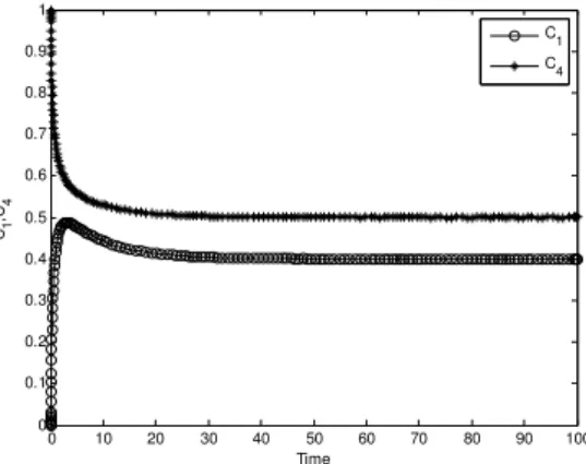
₄ of chemical species. A black circle shows an equilibrium point (0.5, 0.4).

Fig. 3 After completing the transition period, the solution trajectories (

c c

₁

,

₄) goes to steady state after starting from (0,1).

The reduced mechanism with respect to

c c

₁

,

₄ also approaches towards its equilibrium point after

completing its transition period as shown in Fig. 3. Similarly, other possible outcomes can be obtained and they can be shown in the same manner.

0.2 0.3 0.4 0.5 0.6 0.7 0.8 0.9 1 0

0.1 0.2 0.3 0.4 0.5 0.6 0.7 0.8

C

1

C4

Initial trajectory Equilibrium Point

0 10 20 30 40 50 60 70 80 90 100

0 0.1 0.2 0.3 0.4 0.5 0.6 0.7 0.8 0.9 1

Time

C1 ,C4

C₁ C₄

(11)

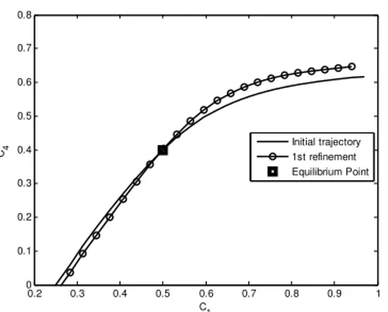
Fig. 4a Refinement of the Initial approximation (measured by QEM) using the method of the Invariant Grid at each point.

Fig. 4b The second refinement (measured by MIG) lays over the first refined trajectory. This means only first refinement gives the exact solution.

Now, refining the initial QEM in Fig. 4 the behaviour of the initial trajectories near an equilibrium point can be seen in Fig. 5.

Fig. 5a Phase flow near the equilibrium point; i.e. lines along with the arrows (vector field) indicate the direction of solution trajectories converging towards the equilibrium point (black circle).

0.2 0.3 0.4 0.5 0.6 0.7 0.8 0.9 1 0

0.1 0.2 0.3 0.4 0.5 0.6 0.7 0.8

C

1

C4

Initial trajectory 1st refinement Equilibrium Point

0.2 0.3 0.4 0.5 0.6 0.7 0.8 0.9 1 0

0.1 0.2 0.3 0.4 0.5 0.6 0.7 0.8

C₁

C4

Initial trajectory 1st refinement 2nd refinement Equilibrium Point

0 0.2 0.4 0.6 0.8 1

0 0.2 0.4 0.6 0.8 1 1.2

(12)

Fig. 5b The phase flow near the equilibrium point along with qem approximation passing through it, i.e (0.5, 0.4).

Now let us discuss another approximation method (SQEM), which not only reduced the system dimension,

but also gave a better approximation as compared to QEM. Thus, according to system (13) and (14) we will

obtain an explicit form

1

0.6043696330 .3721407402

.7599361654

c





y



x

,

2

0.7087392659 1.744281480

1.519872331

c





y



x

,

3

0.5087392659 1.744281480

1.519872331

x

c







y



,

c

₄



y

,

c

₅

  

y

0.5

,

after the selection of vector

v

(slowest left eigenvector) while Jacobin matrix J is measured at an equilibrium

point

.01

.10

0

0 .02

.40

.05

.2

.02

.40

.05

.2

0 .2

.20

.05

.2

0 .2

.20

.05

.2

J









_

















_









_







(15)

delivere the first and second slowest eigenvectors, i.e.,

1

[ -0.1171 -0.2997 0.2997 -0.2178 0.8713]

sl

v



2

[0.0278 0.6522 -0.6522 -0.0935 0.3739]

sl

v



(16)

0.2 0.3 0.4 0.5 0.6 0.7 0.8

0 0.1 0.2 0.3 0.4 0.5 0.6 0.7 0.8

C₁

C4

(13)

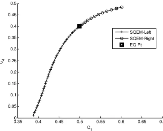
Fig. 6a Initial approximation measured by SQEM started from the equilibrium point (black circle) to both directions, using Euclidean norm 2 2

1 0



ò .

Fig. 6b Refining the initial trajectory (measured by SQEM) with the method of invariant grids shows no difference, i.e. lies over the same approximated curve.

This is now obvious from the above results (refinement Fig. 6b) that SQEM is much better than QEM

approximation. Therefore, one dimensional (SQEM) curve (Fig. 6) can be extended to two dimensions by

applying the method discussed in (3.1). For this purpose, we first take all the measurements (12) with respect

to second slowest vector

v

_sl2 and obtain 1D curve. Then, starting from each grid point of 1D curve, we repeat

the process with vector

v

1_sl. In this way, we obtain a surface, which lies in a phase space as shown in Fig. 7.

0.350 0.4 0.45 0.5 0.55 0.6 0.65 0.7 0.05

0.1 0.15 0.2 0.25 0.3 0.35 0.4 0.45 0.5

C₁

C4

SQEM-Left SQEM-Right EQ Pt

0.350 0.4 0.45 0.5 0.55 0.6 0.65 0.7 0.05

0.1 0.15 0.2 0.25 0.3 0.35 0.4 0.45 0.5

C₁

C4

(14)

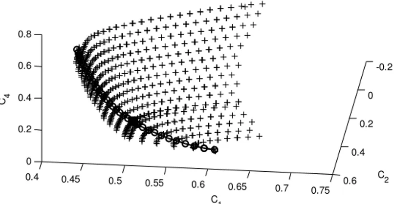
Fig. 7 Initially approximated 1D SQEM (circle line) is further extended (at some of its grid point) for 2D SQEM (black plus) in the second slowest eigen space. The equilibrium is indicated in square and the Euclidean norm in this case is .

Fig. 8a Above figure indicates the variation in eigenvalues (absolute) measured at each grid point (before and after the equilibrium point) with respect to time in case of SQEM.

Fig. 8b Above figure indicates the variation in eigenvalues (absolute) measured at each grid point during the whole process with respect to time measured with respect to SQEM.

0.4 0.45 0.5 0.55 0.6 0.65 0.7 0.75

-0.2

0

0.2

0.4

0.6 0

0.2 0.4 0.6 0.8

C₂

C₁ C4

2 2

0 .5 1 0

 _ _ 

0 0.1 0.2 0.3 0.4 0.5 0.6 0.7 0.8 0.9 1 0.1

0.2 0.3 0.4 0.5 0.6 0.7 0.8 0.9 1

Time

E

ige

n

v

al

ue

v

a

ri

a

ti

on

Fast Eigenvalues Slow Eigenvalues

0 0.1 0.2 0.3 0.4 0.5 0.6 0.7 0.8 0.9 1 0.1

0.2 0.3 0.4 0.5 0.6 0.7 0.8 0.9 1

Time

E

ige

nv

a

lue

v

a

ri

a

ti

on

Fast Eigenvalues Slow Eigenvalues

(15)

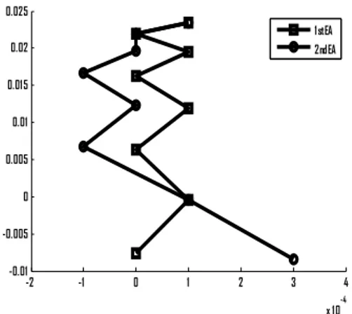
Fig. 9a. Error analysis of the Initial QEM with the MIG are shown for some grid points.

Fig. 9b. In case of SQEM the initial and the refined curve shows no difference.

Table 1 The above tables shows the difference (positive) between the initial (I) and refined (R) values of the eight grid point, which are presented in Fig.9.

Fig.

9a.

|I-R1| |I-R2|

1 0.0234 0.0234

2 0.0219 0.0219

3 0.0195 0.0197

4 0.0163 0.0166

5 0.0119 0.0123

6 0.0063 0.0067

7 0.0004 0.0005

8 0.0076 0.0085

Fig. 9b. 1 2 3 4 5 6 7 8

|I-R1| 0.3606

x 10-03

0.2828

x 10-03

0.2828

x 10-03

0.2236

x 10-03

0.1414

x 10-03

0.1414

x 10-03

0.1000

x 10-03

0

-2 -1 0 1 2 3 4

x 1 0

-4

-0.01 -0.005 0 0.005 0.01 0.01 5 0.02 0.025

1 st EA 2nd EA

-3 -2 -1 0

x 1 0

-4

0 1 2

x 1 0

-4

(16)

IAEES www.iaees.org 7 Conclusion

In this paper, the model reduction is done by employing a slow manifold approach, for which, different

techniques of QEM including steady state approximation and SQEM are used. Although the Intrinsic Low

Dimensional Manifold (ILDM) method, which has been presented by Maas and Pope, 1992 (Maas and Pope,

1994; Maas and Pope, 1992a; Schmidt and Maas, 1996), is one of the efficient methods used to compute SIM.

But the refinement (with MIG) of the QEM, SQEM gives the same results.

The present paper gives an idea that after measuring an equilibrium point, a researcher can move to the

point in a phase space near it and then towards one dimensional curve. After that, two dimensional curves can

be measured while the one dimensional curve lies as a part of it.

By utilizing these approaches, five different species are reduced into some sets of two/three species, which

are included in a model of a particular chemical reaction. The convergence of species also depends on their

transient nature. During the implementation, it is observed that all species have a property that they converge

towards their equilibrium points and then move along it. The equilibrium of ODE’s are stable, which is then

represented by the steady state. The stability of ODE’s can be measured by Lyapunov scalar function

G

while the variation in eigenvalues indicates our selection of slowest variation at each point. This approach can

be utilized for analyzing different chemical reactions associated with species with diverse physical nature.

References

Bothe D, Pierre M. 2010. Quasi-steady-state approximation for a reaction–diffusion system with fast

intermediate. Journal of Mathematical Analysis and Applications, 368(1): 120-132

Chiavazzo E, Gorban AN, Karlin IV. 2007. Comparison of invariant manifolds for model reduction in chemical kinetics. Commun Comput Phys, 2(5): 964-992

Chiavazzo E, Karlin IV. 2008. Quasi-equilibrium grid algorithm: Geometric construction for model reduction. Journal of Computational Physics, 227(11): 5535-5560

Gorban AN, Karlin IV. 2003. Method of invariant manifold for chemical kinetics. Chemical Engineering Science, 58(21): 4751-4768

Gorban AN, Karlin IV. 2005. Invariant manifolds for physical and chemical kinetics. Lecture Notes in Physics,

660: 1-489

Gorban AN, Karlin IV. 2005. Entropy, Quasiequilibrium, and Projectors Field. Springer, Germany

Gorban AN, Karlin IV, and Zinovyev AY. 2004. Invariant grids for reaction kinetics. Physica A: Statistical Mechanics and its Applications, 333: 106-154

Gorban AN, Shahzad M. 2011. The michaelis-menten-stueckelberg theorem. Entropy, 13(5):966-1019

Hangos KM. 2010. Engineering model reduction and entropy-based Lyapunov functions in chemical reaction kinetics. Entropy, 12(4):772-797

Maas U, Pope S. 1994. Laminar flame calculations using simplified chemical kinetics based on intrinsic low-dimensional manifolds. Symposium (International) on Combustion. 1349-1356, Elsevier

Maas U, Pope SB. 1992a. Implementation of simplified chemical kinetics based on intrinsic low-dimensional

manifolds. Symposium (International) on Combustion: 103-112, Elsevier

Maas U, Pope SB. 1992b. Simplifying chemical kinetics: intrinsic low-dimensional manifolds in composition

space. Combustion and Flame, 88(3): 239-264

Marin G, Yablonsky GS. 2011. Kinetics of Chemical Reactions: John Wiley & Sons, USA

(17)

Muhammad Shahzad MS, Muhammad Gulistan, Hina Arif. 2015. Initially Approximated Quasi Equilibrium Manifold. Journal of the Chemical Society of Pakistan, 37: 2

Roy D, and Chaudhari RV. 2005. Analysis of a gas-liquid-liquid-solid catalytic reaction: Kinetics and modeling of a semibatch slurry reactor. Ind Eng Chem Res, 44(25): 9586-9593

Schmidt D, Maas U. 1996. Analysis of the intrinsic low-dimensional manifolds of strained and unstrained

flames. Modelling of Chemical Reaction Systems, Proceedings of an International Workshop, Heidelberg, Germany