Short Communication
Evaluating a Bayesian approach to improve accuracy of individual
photographic identification methods using ecological distribution data
Richard Stafford*, Jane R. Lloyd
Department of Natural and Social Sciences, University of Gloucestershire, Cheltenham, GL50 4AZ, UK
*
E-mail: [email protected]
Received 26 February 2011; Accepted 18 March 2011;Published online 1 April 2011 IAEES
Abstract
Photographic identification of individual organisms can be possible from natural body markings. Data from photo-ID can be used to estimate important ecological and conservation metrics such as population sizes, home ranges or territories. However, poor quality photographs or less well-studied individuals can result in a
non-unique ID, potentially confounding several similar looking individuals. Here we present a Bayesian approach that uses known data about previous sightings of individuals at specific sites as priors to help assess
the problems of obtaining a non-unique ID. Using a simulation of individuals with different confidence of correct ID we evaluate the accuracy of Bayesian modified (posterior) probabilities. However, in most cases, the accuracy of identification decreases. Although this technique is unsuccessful, it does demonstrate the
importance of computer simulations in testing such hypotheses in ecology.
Keywords Bayesian statistics; photo-ID; prior knowledge; site fidelity.
1 Introduction
The identification of individual organisms from natural characteristics, such as spots, stripes or other markings,
can be key to the collection of data while minimising disturbance to the animals (Speed et al.,2007). Such data can be used for estimating population sizes (through modified Capture-Mark-Recapture methods), estimating the territory or home range of individuals or general work on behaviour (Bradbury et al.,2001; Stevick et al.,
2001). Since identification can be time consuming, it can often be best achieved through photographs of the animals, to minimise disturbance of handling time (Reisser et al., 2008; Lloyd et al., 2010). Photographic ID of
individuals has been shown to be successful for numerous species from both marine and terrestrial ecosystems (e.g. Cetaceans–Würsig and Jefferson, 1990; Manta rays– Kitchen-Wheeler, 2010; Turtles–Reisser et al., 2008; Zebras–Peterson, 1972; Leopards–Kelly, 2001). Furthermore, photographs can be taken by individuals other
than trained scientists, and with increasing sophistication of digital cameras and smart phones, photographs can include date, time and position information in the EXIF information, making them a valuable ecological data point (Aanerson et al., 2009; Kirkhope et al., 2010; Stafford et al., 2010).
One problem of photographic ID is that identification can be difficult if there are a large number of similar looking individuals, or if the photograph is of poor quality or from the wrong angle (Culter and Swann, 1999).
particular individual, but still 18% sure it is one of another group of three visually similar individuals – such probabilities are generates by some computer based matching techniques e.g. Hillman et al., 2008).
Incorporating other data, such as site fidelity of an individual, may help increase the probability of identification. Intuitively, if an individual is often seen at a specific site, and a non-conclusive ID is taken at that site, it is more likely to be the commonly seen individual than another individual. As such, incorporating
knowledge of previous sightings of an individual should improve the accuracy of the ID results.
In this study we present a method of modifying probability from a photo-ID based on Bayes’ theorem,
which accounts for the locations of previous sightings and incorporates this as prior knowledge. We predict that use of prior knowledge will increase the probability of a correct identification for an individual with a high level of site fidelity, but decrease the probability of a false identification for a ‘transient’ or migrant individual,
not normally associated with a particular site.
2 Methods
2.1 Computer simulation
A computer simulation was developed in Java, based on the collection of photographs at a series of possible
dive sites. Within a 400×200 pixel grid a total of 10 dive sites (4×4 pixels) were randomly positioned, initially so >50 pixels separated each site (non-clumped sites), and then, in a second group of simulations, from 5
randomly selected sites as above and 5 sites clumped with a 50×50 pixel area (clumped sites), were simulated. In the second simulation, the five clumped sites were analysed both as separate sites, and as a grouped, single site (grouped sites). A series of 10 virtual animals (for example manta rays, whale sharks or terrestrial animals
such as cheetahs, but herein referred to as fish) were simulated within this environment as single pixels. Each fish moved from one pixel to a neighbouring pixel at each of the simulation’s time steps. Which neighbouring pixel (including diagonals) it moved to depended on its current bearing and a modification to this bearing – the
modification being a random number from a normal distribution and mean of zero as per Stafford et al. (2007). By altering the standard deviation of this distribution, or by including a 180º turn after a certain number of
time steps (Table 1), different levels of site fidelity could be created.
If the fish moved into a ‘dive site’ then there was a 50% chance of a photograph of the fish being taken, and an ID being made on that photograph – based on not every sighting being successfully photographed, as is the
case with any photo-ID project. The ID was made with a confidence range set as an adjustable parameter (in this case ID probability was defined as a random number from a normal distribution with mean=0.9, 0.7 or 0.5
and S.D.=0.2, with limits between 0 and 1). Each fish was in a group of other ‘visually similar’ fish, with which it could be easily visually confused (Table 1). Therefore if a random number (uniform, between 0 and 1) was higher than the assigned ID probability, the fish identified was given to a different randomly determined
fish from the visually similar grouping (essentially a mis-identification). Note, behavioural groupings and visual grouping were not identical (Table 1).
As such, the simulation outputted an identification for an individual (based on the above process), with a probability of identification (p which varied between 0 and 1). Also, probability of similar individuals in the group was calculated as per equation (1):
r = (1-p) / (n-1), (1)
Details of the dive site and time of sighting were also given, as was the true identity of the fish. Simulations were run for a total of 48,000 time steps, giving around 100 sightings per replicate run. For clumped and
grouped sites (see above) the predefined ID confidence range was of mean 0.7 (S.D.=0.2). Non-clumped sites were tested with all three ID probabilities (mean=0.9, 0.7 and 0.5, S.D.=0.2 in all cases).
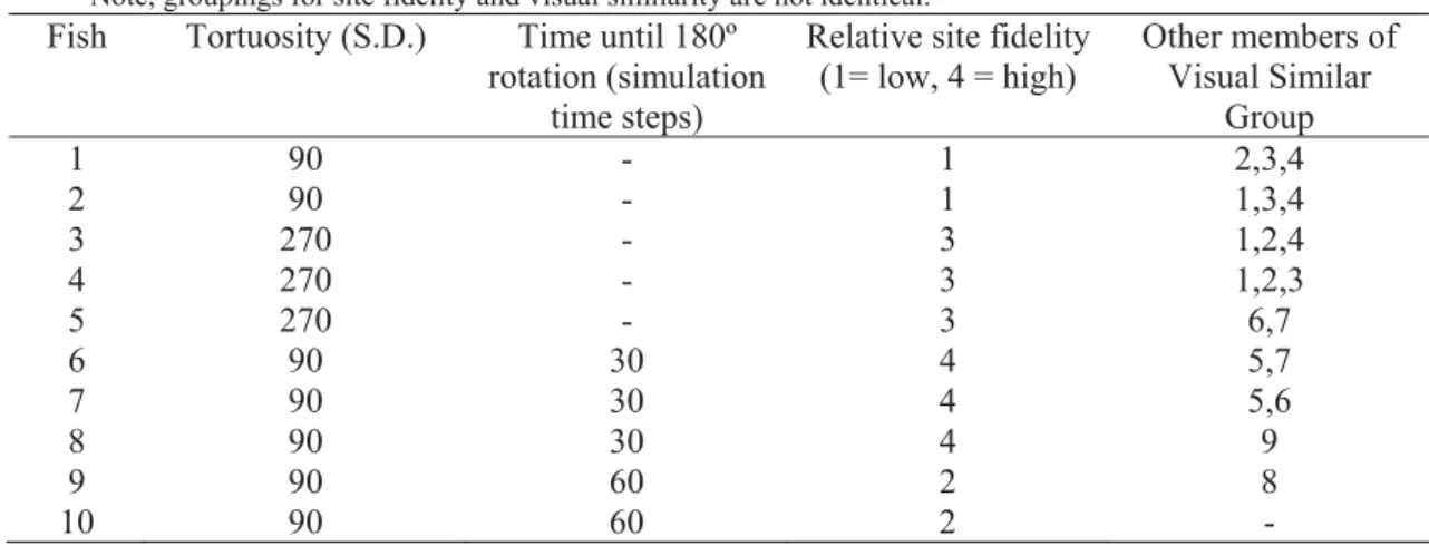
Table 1 Simulation parameters and behavioural and visual groupings of different of simulated fish. Note, groupings for site fidelity and visual similarity are not identical.
Fish Tortuosity (S.D.) Time until 180º rotation (simulation
time steps)
Relative site fidelity (1= low, 4 = high)
Other members of Visual Similar
Group
1 90 - 1 2,3,4
2 90 - 1 1,3,4
3 270 - 3 1,2,4
4 270 - 3 1,2,3
5 270 - 3 6,7
6 90 30 4 5,7
7 90 30 4 5,6
8 90 30 4 9
9 90 60 2 8
10 90 60 2 -
2.2 Bayesian modification
Bayesian analysis was conducted using an R script file (R Core Development Team, 2007). Whenever an individual was recorded at a given site, details of the site it was seen at were taken. For a first sighting, the
probability of identification of a given fish at a given site was recorded as the probability p (as definedin the section above). Over time, therefore, a database was built up of probabilities of given fish at given sites. For subsequent sightings of a given fish at a given site, the posterior probability of correct identification was
modified using the Bayesian equation (equation (2)):
Ppost=p.Qf1,s /(p.Qf1,s +r.Qfx,s), (2)
wherep and r are as per equation 1, and Qf1,sandQfx,s were the priors of fish 1 at site s, and fish x (where x
runs from 2 to n) at site s respectively.
Equally, the probability of seeing the other fish in the visually similar grouping was also modified
accordingly using the same equation, and subsequently Ppost became Qf1,s. The process was repeated with each sighting and processed in the order in which the sightings occurred.
Details of the overall percentage increase in correct identifications, and the overall decrease in
mis-identification was calculated for each of the cases listed above (different probability of mis-identification rates, and different spatial distributions and groupings of sites).
3 Results
In a minority of cases, Bayesian modification of ID probabilities did increase, allowing a transparent process
to increase ‘certainty’ of sighting ID, based on knowledge of the behaviour and biology of the organisms (Table 2). However, while it may be predicted that such an increase would be found for species with high site
cases, modification of probabilities was reversed from what was expected. Correctly identified individuals had lower probability after Bayesian modification and incorrectly identified individuals had higher probability
(Table 2).
Table 2 Percentage changes between initial probability of ID and modified Bayesian probability of ID. Data is given for different initial levels of probability of recognition, both for all fish, and split between behavioural groups of fish given in Table 1. Different dispersal and categorisation of sites is also given as defined in Methods. Negative numbers indicate a change in probability in the ‘wrong’ direction, for example, a reduction in the probability of identification for the correct fish, or an increase in probability of identification for a mis-identified fish.
ID probability
Grouping of Sites
Behavioural Grouping (fish
numbers)
% increase in probability of correctly identified
individuals
% decrease in probability of wrongly identified
individuals
0.9 Random All -1.7 8.1
0.7 Random All -2.3 -4.9
0.5 Random All 11.1 -17.0
0.7 Clumped All -3.4 -8.3
0.7 Grouped All 2.7 -8.1
0.9 Random 1,2 -3.0 4.0
0.9 Random 3,4,5 -7.1 3.5
0.9 Random 6,7,8 1.6 26.8
0.9 Random 9,10 -0.7 0.6
0.7 Random 1,2 0.9 -0.7
0.7 Random 3,4,5 -7.2 -36.8
0.7 Random 6,7,8 -4.0 -10.0
0.7 Random 9,10 5.1 25.0
0.5 Random 1,2 -9.1 -37.8
0.5 Random 3,4,5 6.2 3.7
0.5 Random 6,7,8 3.6 4.6
0.5 Random 9,10 36.0 39.6
0.7 Clumped 1,2 -2.4 5.5
0.7 Clumped 3,4,5 -4.4 12.0
0.7 Clumped 6,7,8 -6.0 -2.1
0.7 Clumped 9,10 1.5 -46.2
0.7 Grouped 1,2 1.2 1.2
0.7 Grouped 3,4,5 -0.4 0.8
0.7 Grouped 6,7,8 6.2 0.8
0.7 Grouped 9,10 6.0 -41.8
4 Discussion
Bayesian statistics has increased in popularity, especially in the ecological sciences, in recent years (Link and
Barker, 2010). The reasons for such an increase in popularity are clear – ecology frequently obtains data from different, but related sources, for example, on the same species, but in different locations, or on several closely related species. As such, the use of existing knowledge as priors can be very useful – potentially reducing the
number of samples needed to be taken to ensure a suitably powerful statistical analysis. However, arguments against Bayesian approaches tend to be centred on the selection of prior values, and their often arbitrary nature
(Wilson, 2010). The use of biologically relevant data, such as used here, should result in more meaningful priors. Essentially, here, two sets of data are being combined, one relating to biological knowledge of individuals (based on previous sightings), and the second being related to new sightings. However, from the
In the current case, the Bayesian approach would essentially mimic human intuition. Seeing an individual in the same place on countless occasions would result in a likely increase in the likelihood of identifying an
individual, of which you were unsure of, as being the commonly seen individual. However, counter intuitively, this appears not to be the case, especially when similar looking transient species – or initial mis-identification of individuals can occur.
These results are important, even if describing a process that does not work. Given the intuitive nature of such a technique, it would be logical to apply such a process in field studies. However, it is only through the
process of computer simulations that the ‘real’ individual was known for each sighting, and therefore the accuracy of the Bayesian modification can be calculated. While statistical approaches to improve precision of citizen science reporting, or improve identification rates of photograph ID are important (Stafford et al., 2010),
it is often only through computer-based simulation that evaluation of such techniques involving uncertain data can be conducted.
References
Aanensen DM, Huntley DM, Feil EJ, al-Own F, Spratt BG. 2009. EpiCollect: linking smartphones to web
applications for epidemiology, ecology and community data collection. PLoS One, 4: e6968
Bradbury RB, Payne RJH, Wilson JD, Krebs JR. 2001. Predicting population responses to resource management. Trends in Ecology and Evolution, 16: 440-445
Culter TL, Swann DE. 1999. Using remote photography in wildlife ecology. Wildlife Society Bulletin, 27: 571 -581
Hillman GR, Trask KD, Sweeney K, Davis AR, Koski WR, Mocklin J, Rugh DJ. 2008. Photo-identification software for bowhead whale images. Paper SC/60/BRG24 International Whaling Commission Scientific Committee, Santiago, Chile
Kelly MJ. 2001. Computer-aided photograph matching in studies using individual identification: an example from Serengeti Cheetahs. Journal of Mammalogy, 82: 440-449
Kirkhope CL, Williams RL, Catlin-Groves CL, Rees SG, Montesanti C, Jowers J, Stubbs H, Newberry J, Hart AG, Goodenough AE, Stafford R. 2010. Social networking for biodiversity: the BeeID project. In: Proceedings of the iSociety Conference (Ed. CA Shoniregun). London
Kitchen-Wheeler AM. 2010. Visual identification of individual manta ray (Manta alfredi) in the Maldives Islands, Western Indian Ocean. Marine Biology Research, 6: 351-363
Link WA, Barker RJ. 2010. Bayesian Inference with Ecological Applications. Academic Press, London Lloyd JR, Maldonado MA, Hart AG, Stafford R. 2010. Development of a key to identify individual green
turtles from photographic records. 30th Annual Symposium on Sea Turtle Biology and Conservation, Goa,
India
Peterson JC. 1972. An identification system for zebra. East African Wildlife Journal, 10: 59-63
R Development Core Team. R: A language and environment for statistical computing. R Foundation for Statistical Computing, Vienna, Austria, 2007 (http://www.R-project.org)
Reisser J, Proietti M, Kinas P, Sazima I. 2008. Photographic identification of sea turtles: method description
and validation, with an estimation of tag loss. Endangered Species Research, 5: 73-82
Speed CW, Meekan MG, Bradshaw CJA. 2007 Spot the match: wildlife photo-identification using information
theory. Frontiers in Zoology, 4: 2
Stafford R, Davies MS, Williams GA. 2007. Computer simulations of high shore littorinids predict small-scale spatial and temporal distribution patterns on real rocky shores. Marine Ecology Progress Series,
Stafford R, Hart AG, Collins L, Kirkhope CL, Williams RL, Rees SG, Lloyd JR Goodenough AE. 2010. Eu-social science: the role of internet Eu-social networks in the collection of bee biodiversity data. PLoS ONE, 5:
e14381
Stevick PT, Palsbøll PJ, Smith TD, Bravington MV, Hammond PS. 2001. Errors in identification using natural markings: rates, sources, and effects on capture recapture estimates of abundance. Canadian Journal of
Fisheries and Aquatic Science, 58: 1861-1870
Wilson MA. 2010. Bayesian Model Uncertainty and Prior Choice with Applications to Genetic Association
Studies (Ph.D. Dissertation). Duke University, USA