A Bayesian Approach to Predicting Water Supply and Rehabilitation of Water Distribution Networks

A Bayesian Approach to Predicting Water Supply and

Rehabilitation of Water Distribution Networks

Abdelaziz Lakehal

Department of Mechanical Engineering Mohamed Chérif Messaadia University P.O. Box 1553, Souk-Ahras, 41000, Algeria

Fares Laouacheria

Abstract—Water distribution network (WDN) consists of several elements the main ones: pipes and valves. The work developed in this article focuses on a water supply prediction in the short and long term. To this end, reliability data were conjugated in decision making tools on water distribution network rehabilitation in a forecasting context. The pipes are static elements that allow the transport of water to customers, while the valves are dynamic components which perform ensure management of water flow. This paper presents a Bayesian approach that allows management of water distribution network based on the evaluation of the reliability of network components. Modeling based on a Static Bayesian Network (SBN) is implemented to analyze qualitatively and quantitatively the availability of water in the different segments of the network. Dynamic Bayesian networks (DBN) are then used to assess the valves reliability as function of time, which allows management of water distribution based on water availability assessment in different segments. Finally an application on data of a fraction of a distribution network supplying a town is presented to show the effectiveness and the strong contribution of Bayesian networks (BN) in this research field.

Keywords—Water distribution network (WDN) management; Rehabilitation; Pipes and valves reliability; Bayesian Networks (BN); Water supply

I. INTRODUCTION

The water distribution networks (WDN) are underground infrastructure; they are intended for water supply to the consumers at working pressure in a specific range. These networks mainly include pipes, connection of water, metering systems and valves. Today, water grids are made up primarily of polyethylene pipes. At the downstream of these networks are situated individual or collective connections themselves shall be constructed of polyethylene or other equivalent material.

Through this article we will try to give a contribution to WDN management by assessing their reliability. The availability of water in the WDN depends on the availability of the pumping system, water quality, the mechanical behaviour of network components, and hydraulic parameters. All these parameters contribute to the assessment and the reliability analysis of WDN. Ostfeld [1] defined the reliability on the basis of the water quality by the fraction of the delivered quality. Kansal and Arora [2] defined the reliability on the basis of the water quality by the proportion of time in which the network was able to provide the desired water quality. The above two parameters are based on the proportion

of time during which the network provided high-quality of water. Kansal and Arora [2] proposed a widely accepted methodology for analyzing the reliability of WDN based on the water quality assessment using two parameters: the reliability of hydraulic system and the quality of water. These reliability parameters: hydraulic and water quality described as well the reliability of WDN. The major disadvantage in obtaining these parameters is highly related on the mathematical modelling methodology [3]. Quantitatively, the reliability of a water distribution system can be defined as the complement of the probability that the system fails, a failure is defined as the inability of the system to provide consumers with a drinking water (quality and continuity of service). Two types of events can cause the failure of a water distribution system: the failure of the system components (eg tubes and / or hydraulic control elements) and / or demand (transportation of the desired quantities of water to the desired pressure at desired appropriate locations and at desired appropriate times). These definitions show that the reliability of WDN can be classified into two main categories: topological and hydraulic reliability [4].

The above paragraphs show that the management of a WDN is based primarily on the quality, topological reliability and hydraulic reliability. In the following, we focus on the topological reliability and specifically the mechanical reliability of the components of the WDN, the failure of one of these elements can leave a fraction of the WDN out of service and consequently interrupting the water supply of a population.

Several authors have based their studies in the field of WDN on the reliability assessment by artificial intelligence methods either in the design phase [5] or the operation phase [6]. The methodology presented below is based on the assessment of the water availability in the WDN on the basis of the reliability modelling of pipe and valves by using Bayesian network (BN).

II. THE BAYESIAN MODELS

defined a priori by measurement, or following investigations (expert opinion). The causes and consequences are uncertain or "stochastic" variables. They are discrete but there are belief scenarios where analysis involving continuous variables. In situations of uncertainty where expert knowledge and measurement data is incomplete, the use of posterior observations by a Bayesian approach reduces and eliminates this uncertainty.

In Bayesian methods, a priori information, the likelihood and a posteriori information are represented by probability distributions. A priori probability represents the probability distribution of knowledge on a variable before that the parameter it represents is observed. The likelihood is a function of parameters of a statistical model reflecting the possibility of observing a variable if these parameters has a value. A posteriori probability is the conditional probability of the data collected by combination of prior probability and likelihood via Bayes' theorem [7].

In a BN, dependence and causality is represented by edges. An edge between two variables implies a direct dependence between these two variables: one is called the parent, and the other named child. In a Bayesian model, the behaviour of the child variable should be given in view of the behaviour of its parent or parents (if there are several). To do this, each node in the network has a conditional probability table (CPT). A CPT associated with a node allows quantifying the effect of the parent node on that node: it describes the probabilities associated with child nodes according to the different values of the parent nodes. For root nodes (without parents), the probability table is no longer conditional and gives them a priori probabilities [8].

The BN prohibit child dependencies to parents. Thus, the set of variables and edges will form a directed (edges have a

sense) and acyclic graph (no cycle in the graph). Therefore, a BN (Figure 1) is defined by a directed acyclic graph (DAG) as [9]:

∏ (1)

Where C (Vi) is the set of parents (or causes) of Vi in DAG.

Fig. 1. Example of a simple Bayesian network

III. BAYESIAN MODEL DEVELOPMENT FOR WATER SUPPLY PREDICTION

A. Modeling with Static Bayesian Network

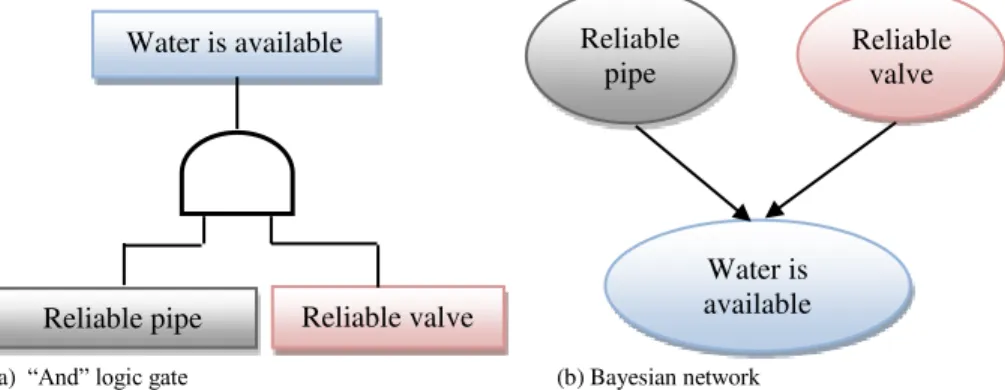
Modelling with BN is similar to that of the fault tree [10]. The fault tree is a systematic and comprehensive approach to determine the sequence and combinations of events that could lead to a top event taken as a reference (Figure 2.a). Whatever the nature of the basic elements identified, fault tree analysis found on the basis that the events are independent. In a BN, the connections between events will be represented by edges that reflect the dependence between these events, and cause-effect relationship. The different types of events will be represented by nodes on the basis that basic events will be the input nodes for the model (Figure 2.b).

The availability of water in a section depends on the reliability of the pipe and that of the valve. A BN models the events with the nodes, while the distinction between the various logic gates of a fault tree is made by adjusting the CPT [10].

(a) “And” logic gate (b) Bayesian network Fig. 2. Conversion of fault tree into Bayesian network

B. Modelling with Dynamic Bayesian Network

A BN is a modelling tool that treats problematic where the variable is static. In this field, each variable has a unique and fixed value. Unfortunately, this static variable hypothesis does not always take. As many domains exist where the variables are dynamic and reasoning in time is necessary such as dynamic systems. Dynamic Bayesian Networks (DBNs) are graphical models allowing to compactly representing the inherent uncertainties in dynamic systems evolving over time. The BNs and DBNs have given a strong contribution in the

illustrative examples, we can cite the work of [11] for modelling reliability of a complex system using BNs, and [12] for modelling reliability by DBNs.

In the framework of this study we will use the DBN for assessing the reliability of the valves and therefore predicting the different supply situations of the various sections. In order to master the water supply, it is necessary to control and monitor over time the evolution of variables (water availability) for each segment of the WDN. To achieve this objective the idea is to infer, what is the possibility for Water is available

Reliable pipe Reliable valve

Reliable pipe

Water is available

opening sequences of the valve. In this case the random hidden variable is (water availability)t with two state (true)

and (false), and the observed variable is (the status of the

valve)t and the satisfaction of these suppositions is modelled

by the dependencies between all variables in the model that is given by the BDN in Figure 3:

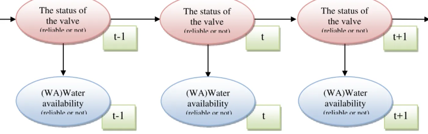
Fig. 3. Modelling of water supply of a network segment by Dynamic Bayesian Network

In Figure 3, the fact indicate an edge between the two variables (water availability)t and (the status of the valve)t, this

means that the availability of water depends on the status and reliability of the valve at time t and similarly, the reliability of the valve at time t depends on its reliability at time t-1. From this DBN it is possible to calculate the most recent a posteriori distribution of the variable (water availability)t by filtering,

also it is possible to calculate the a posteriori probability of the variable (water availability)t+n in a future time, where n the

number of time steps, such as:

⁄ ∏ ⁄ (2) IV. APPLICATION AND DISCUSSION

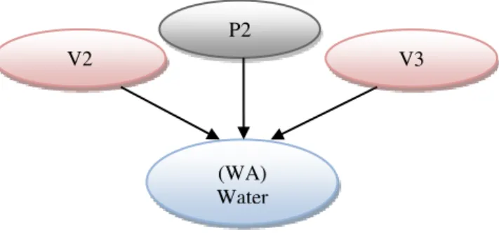
The data used in the examples that will be presented in the rest of this paper concern a WDN supplying a city. There are two architectures for networks either meshed network (or ringed) or network in a radial arrangement. In the first case, the network segment is controlled by one valve, so the availability of water in the framework of this study is mainly dependent on the reliability of the pipe and of the valve (Figure 4.a). In the second case the water availability depends essentially on the reliability of piping and block valves (in the case study there are two valves) (Figure 4.b).

The modelling of the failure rate (breaks or leaks) by segment requires a significant history of maintenance data. Alternatively, the approach of the entire WDN is insufficient because it does not allow to plan and implement short-term actions. However, the design of reliable models must be adapted with the available data and analysis must be done on a scale segments according to several criteria: material, diameter, when it was laid, flow, pressure, and road.

Pipe failure rates in a distribution system can be determined from historical failure/repair data. In the case where historical failure data indicate a deteriorating network, a classical reliability assessment of the network can be done using Poisson process for modelling the pipe failures. In this case, the reliability measure is based on individual pipe failure probabilities. Here, the probability of failure of an individual pipe is given by:

₍₃₎ Where:

P: Probability of failure  : Failure rate

t: Time Network architecture Associated Bayesian network

(a) Radial network

t+1

availability (reliable or not)

t

(WA)Water availability (reliable or not)

t-1

(WA)Water availability (reliable or not)

t-1

the valve (reliable or not)

t

the valve (reliable or not)

t+1

the valve (reliable or not)

Valve V1

Pipe P1 To customers

P1 reliable

(WA) Water

(b) Mesh network

Fig. 4. Bayesian network models for the two network architectures

An estimation of (t) by time slice is determined by the following calculation:

(4) Where:

ni : the number of failed during Δti

Ni : the number of survivors at the beginning of the slice ti

Δti = ti+1-ti : the observed time interval

By applying the formula (4) to the WDN (t) is given by:

∑

∑ : Number of failures/ 100m/ year (5) Where:

ni : the number of observed failures on segment i

Li : length corresponds to each segment i (in meters)

Δti : the observation period for each segment i (in year)

The proposed Bayesian approach gives the probability of failure of an individual pipe from the equation (1). For a leak on the pipeline (LP), the reliability decreases (RP), provided that P (reliability of pipe) ≠ 0:

⁄ ⁄ (6) Bayes' theorem can reverse the probabilities. That is to say, if we know the reliability of the pipe as a consequence of leaking pipe, observing the effects allows estimating the probability of failure.

⁄ ⁄ (7) The definition of a priori probabilities is the most difficult step in the model development; it is based on knowledge held

by experts or the feedback. It also requires special attention because the results obviously depend on the available data and on some hypothetical models.

A valve is defined as a dynamic mechanical device by which the flow of fluid may be started, stopped, or regulated by a movable part that opens or obstructs passage. Control valves are used to regulate flow or pressure at different points of the system by creating headless or pressure differential between upstream and downstream sections. The mission of isolation valves is to isolate a portion of the system whenever system repair, inspection, or maintenance is required at that segment; in the following we are interested in the isolation valves. The reliability of valves themselves has not been implicitly or explicitly incorporated in reliability assessments to date. Perhaps the main reason for this is that the human factor is the most important factor in determining their reliability. The more frequent the valve exercising programs, the greater the chance that they will operate when needed.

The water availability depends on the state of the valve. Following a closing valve, if it will not open there will be no water. From Equation (2) it’s possible to define the valve reliability as a function of the valve failure (Valve won't open).

⁄ ∏ ⁄ (8) For experimentally determine the failure rate  which corresponds to the probability of having failure in the time intervals constituting the life cycle of the studied WDN, the historical files and the formula (5) are used. Table 1 gives the failure rates (leaking pipe) for pipes P1 and P2, with two states (true) and (false) and the valves V1, V2, and V3 with regard to fault: the valve not open (Valve won't open), with two states (true) and (false).

To customers

Valve V2 Valve V3

Pipe P2

P2 reliable

(WA) Water

V3 reliable V2

TABLE I. APRIORI PROBABILITIES

Element Failure State Probability

P1 Leaking pipe (LP1) True (T)  = 0.136 P2 Leaking pipe (LP2) True (T)  = 0. 213 V1 Valve won't open (VWO1) True (T)  = 0.057 V2 Valve won't open (VWO2) True (T)  = 0.026 V3 Valve won't open (VWO3) True (T)  = 0.033

T : True, F : False

DBN encodes the joint probability distribution of a time-evolving set of variables V (t) = {V1 (t),…, Vi (t)}. If we consider t time slices (time step) of variables, the DBN can be considered as a "static" BN with T × i variables. In this context the probability of supplying (water availability WA) the subscribers connected to the network of Figure 4.a is calculated as follows:

P (WA=T) = P (WA=T / LP1=T, VWO1=T)  P (LP1=T)  P (VWO1=T) +

P (WA =T / LP1=T, VWO1=F)  P (LP1=T)  P (VWO1=F) +

P (WA =T / LP1=F, VWO1=T)  P (LP1=F)  P (VWO1=T) +

P (WA =T / LP1=F, VWO1=F)  P (LP1=F)  P (VWO1=F)

Using the data collected in the table 1 we find: P (WA=T) = 0  0.136  0.057 + 0  0.136  0.943 + 0  0.864  0.057 +

1  0.864  0.943 P (WA=T) = 0.814

As soon as the number of nodes increases the calculations become difficult. Similarly calculations are made more

complicated for modelling the dynamic behaviour of valves with DBN. To relax these constraints a program was used.

Table 2 and Table 3 give the conditional probability tables for the two network architectures.

TABLE II. CONDITIONAL PROBABILITY TABLE FOR RADIAL NETWORK

VWO1 T F

LP1 T F T F

Water Availability (WA) True (T) 0 0 0 1

False (F) 1 1 1 0

TABLE III. CONDITIONAL PROBABILITY TABLE FOR MESH NETWORK

VWO2 T F

VWO3 T F T F

LP2 T F T F T F T F

Water Availability (WA)

True (T) 0 0 0 1 0 1 0 1

False (F) 1 1 1 0 1 0 1 0

The interpretation of CPTs is as follows: for the first architecture, if the valve does not open, water is not available, and also if the pipe is faulty, water is unavailable. One of these two conditions implies that water is not available (OR gat in Fault tree analysis). For the second architecture, water is available, if at least one of the valves opens and pipe is not leaking (reliable pipe).

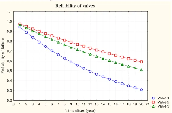
The valves have a dynamic behaviour; however, and from equation (8) the temporal probability distributions of the three valves V1, V2, and V3 are shown in Figure 5.

Reliability of valves

Valve 1 Valve 2 Valve 3

0 1 2 3 4 5 6 7 8 9 10 11 12 13 14 15 16 17 18 19 20 21

Time slices (year) 0,2

0,3 0,4 0,5 0,6 0,7 0,8 0,9 1,0 1,1

Pr

ob

abil

it

y

of

f

ai

lu

re

Applying formula (2) and on the basis of CPTs shown in Tables 2 and Table 3, the water availability probabilities as a function of time are obtained. The results are shown in

Figure.6 and Figure 7, they depend on the reliability data of the valves V1, V2, V3, the two segments of network P1, and P2 and also the two architectures (defined by CPTs): Water supply prediction

0 1 2 3 4 5 6 7 8 9 10 11 12 13 14 15 16 17 18 19 20 21

Time slices (year) 0,2

0,3 0,4 0,5 0,6 0,7 0,8 0,9

Wat

er

avai

labi

li

ty

Fig. 6. Water supply for radial network

Water supply prediction

0 1 2 3 4 5 6 7 8 9 10 11 12 13 14 15 16 17 18 19 20 21

Time slices (year) 0,60

0,62 0,64 0,66 0,68 0,70 0,72 0,74 0,76 0,78 0,80

Water availability

Fig. 7. Water supply for meshed network

This section presents predictive results on water supply; results were based on the reliability of the pipes and valves (Figure 6 and Figure 7). From the results of the developed model it’s possible to easily extract information and transform them into quantitative and qualitative data. This approach allows predicting the behaviour of WDN gives the possibility

of a predictive management of water supply and anticipates failures of network elements. On the other hand, it is possible from the developed Bayesian approach to simulate the maintenance actions and investment reflections.

meshed architecture, but the probability that the mesh network is supplied is 78.63% for the first year. Lower value than that of the radial network (81,74%). This is due mainly to the failure rate (P2) which is higher than (P1). After 10 years of service, the supply from the radial network is found with a probability of 48.04%, low value. After the same period the subscribers connected to the mesh network will have a water supply probability equal to 73.50%, higher value compared with that of the network in a radial arrangement. Now, after 20 years the radial network is at the end of service life, on the other hand, the mesh network is still profitable (a water supply probability greater than 62%).

From these results it is also possible to define a plan of action for the rehabilitation of WDN. For example, if the probability of 60% is fixed as the threshold value on the probability of water supply for the rehabilitation of the WDN, it is necessary to provide the rehabilitation for the radial network from the seventh year, whereas for the mesh network rehabilitation is not needed for the 20 years.

The proposed Bayesian model has a great interest compared to the Poisson model. It classifies sections with low failure rates, or who have not experienced failures (failure rate equal to 0) with similar sections. When new information is available on the individual failure rate, the results will be updated by inference without increasing the calculation time.

In order to expand the study by taking into account hydraulic reliability and reliability-based quality (the level of chlorine in the water) it is possible to develop the model by adding the quality and hydraulic parameters as input variables in the model. The same goes with adding new information; add a new variable in Bayesian models is not difficult and the inference process will not take a significant time for calculating the new a posteriori probabilities.

A WDN operates as a system of dependent components (valve, pipe, individual and collective water connection). The hydraulics of each component is relatively straightforward; however, these components depend directly upon each other and as a result affect each other’s performance. The purpose of the Bayesian analysis is to determine how the systems perform hydraulically under various demands and operating conditions. In this paper, a segment of network has been studied. If the study is generalized over the entire network with its multitude of valves; pipe and connections, the results found in the examples are used for the following situations:

 Evaluation of WDN reliability

 WDN performance and operation optimization: prioritize actions and supporting any strategic decisions.  Determination of rehabilitation priorities

 Design of a new WDN: best choice of the network design (radial or mesh network) by considering the reliability as a central element in this design in parallel with the hydraulic elements

 Modification and expansion of an existing WDN: the implantation and the management of the boundary

valve in the network is essential in maintaining the integrity of the hydraulic structure

 Preparation for maintenance: optimizing the systematic and predictive maintenance

Analysis of WDN malfunction: such as water connection breaks, leakage, valve failure

V. CONCLUSION

In this paper, the Bayesian approach presented will be a useful tool in the decision-making process. The model developed in this work helps operators of WDN to assess the water availability as function of time which allows a predictive management of water supply. The use of DBN is due to the dynamic character of flow control components which are valves. The Bayesian approach used for modelling the reliability of pipe which has experienced failures, pipes without failures, and valves, represents a new and unique tool for the three cases compared to existing models in the literature. The found results have contributed greatly to estimating in a realistic and practical estimation of foreseeable demand to improve management of the quantities of water and to improve the operational capability of operation and maintenance services. Also in the operation of WDN and in general, maintenance and investment actions must be included in the time. To do this, the DBNs are powerful simulation tools of the impact of these actions on the future management of WDN.

In the future work, we will look forward to developing the model by taking into account the hydraulic reliability and the reliability based quality on the one hand and on the other hand by considering the human factor that also represents an influence factor in determining the reliability of the valves.

REFERENCES

[1] A. Ostfeld, “Reliability analysis of water distribution systems,” J. Hydroinform. vol. 6, 4, 281–294, 2004.

[2] M.L. Kansal, and G. Arora, : Water quality reliability analysis in an urban distribution network, ” J. Indian Water Works Assoc. vol. 36, 3, 185–198, 2004.

[3] R. Gupta, S. Dhapade , S. Ganguly and P.R. Bhave, : Water quality based reliability analysis for water distribution networks,” ISH Journal of Hydraulic Engineering. vol. 18, 2, 80–89, 2012.

[4] A. Ostfeld, : Reliability analysis of regional water distribution systems,” Urban Water. vol. 3, 4, 253–260, 2001.

[5] T. D. Prasad, S.H Hong, and N. Park, : Reliability based design of water distribution networks using multi-objective genetic algorithms,” KSCE Journal of Civil Engineering. vol. 7, 3, 351-361, 2003.

[6] V. Kanakoudis, S. Tsitsifli, : Water pipe network reliability assessment using the DAC method,” Desalination and Water Treatment. vol. 33, 97–106, 2011.

[7] A. Darwiche, Modeling and Reasoning with Bayesian Networks. Cambridge University Press, 2009.

[8] Jensen, F, V. An Introduction to Bayesian Networks. UCL Press; 1996. [9] P. Naim, P.H. Wuillemin, P. Leray, O. Pourret, and A. Becker, :

Réseaux bayésiens. 2 ed. France: Eyrolles; 2004.

[11] H. Boudali, and J.B. Dugan, : A discrete-time Bayesian network reliability modeling and analysis framework,” Reliability Engineering and System Safety. vol. 87, 3, 337-349, 2005.