ANALYSIS OF BAYESIAN CLASSIFIER ACCURACY

© 2013 Science Publications

doi:10.3844/jcssp.2013.1487.1495 Published Online 9 (11) 2013 (http://www.thescipub.com/jcs.toc)

Corresponding Author: Felipe Schneider Costa,Departamento de Informática e Estatística, Universidade Federal de Santa Catarina, Florianópolis, Brazil

ANALYSIS OF BAYESIAN CLASSIFIER ACCURACY

1

Felipe Schneider Costa,

2

Maria Marlene De Souza Pires and

Silvia Modesto Nassar

1

Departamento de Informática e Estatística, Universidade Federal de Santa Catarina, Florianópolis, Brazil 2

Centro de Ciências da Saúde, Universidade Federal de Santa Catarina, Florianópolis, Brazil

Received 2013-08-27, Revised 2013-09-24; Accepted 2013-09-26

ABSTRACT

The naïve Bayes classifier is considered one of the most effective classification algorithms today, competing with more modern and sophisticated classifiers. Despite being based on unrealistic (naïve) assumption that all variables are independent, given the output class, the classifier provides proper results. However, depending on the scenario utilized (network structure, number of samples or training cases, number of variables), the network may not provide appropriate results. This study uses a process variable selection, using the chi-squared test to verify the existence of dependence between variables in the data model in order to identify the reasons which prevent a Bayesian network to provide good performance. A detailed analysis of the data is also proposed, unlike other existing work, as well as adjustments in case of limit values between two adjacent classes. Furthermore, variable weights are used in the calculation of a posteriori probabilities, calculated with mutual information function. Tests were applied in both a naïve Bayesian network and a hierarchical Bayesian network. After testing, a significant reduction in error rate has been observed. The naïve Bayesian network presented a drop in error rates from twenty five percent to five percent, considering the initial results of the classification process. In the hierarchical network, there was not only a drop in fifteen percent error rate, but also the final result came to zero.

Keywords: Bayesian Network, Entropy, Feature Weighting, Mutual Information, Small Sample Set

1. INTRODUCTION

Many tasks, including fault diagnosis, pattern recognition and forecasting can be seen as classification (Cheng and Greiner, 1999). The classification is a base task in data analysis and pattern recognition which requires the construction of a classifier, that is, a function that assigns a class tag to examples described by a set of variables. The inference of classifiers on data sets with pre-classified cases is a central problem in machine learning. Several approaches to this problem are based on functional representations such as decision trees, neural networks and rules (Friedman et al., 1997).

The use of statistical tests to identify relationships and build the graphical structure of a network has been frequently used. Cheng and Greiner (1999) use a process of selecting variables (and discarding others), as well as

using the mutual information function to quantify dependency relations between variables in a data model. Zhang (2004) proposes a new explanation on the excellent performance of naïve Bayes classifier by introducing the concept of local dependence. In the study by (Lee et al., 2011) weights are assigned to the variables of the data set by using the Kullback-Leibler measure.

However, most of the work already developed did not care with the assignment process of categories (discretization) for values of variables in the data set. It is easy to see that attributes with boundary values can compromise the classification task, since changing the category of a variable can change the value of the output variable.

allocation of categories to the variable values on training cases. As regards to model variables that were used to construct the network structure, a process of variable selection was applied by using a chi-squared test to verify the association between two variables. In order to control the influence of each variable in calculating probability a posteriori, variable weights were calculated using the mutual information function.

Therefore, by acting in the process of categorizing values of the data set, in selecting variables that form the network structure and in reducing or increasing how each variable affects the output class, it is expected to result in a performance increase by the Bayesian classifiers utilized.

1.1. Theoretical Background

1.1.1. Bayesian Networks

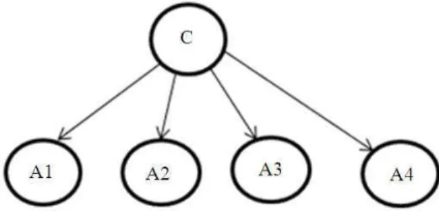
Bayesian networks (Pearl, 1988) are powerful tools for knowledge representation and inference under conditions of uncertainty that have only been considered classifiers upon the discovery of the naïve Bayes classifier. Surprisingly effective, the naïve Bayes classifier is essentially a simple Bayesian network in which every variable is considered independent of one another, given the classification node (Cheng and Greiner, 1999).

A Bayesian network is a systematic way to represent relationships between the independent variables through a data structure (directed graphs), in which each node is labeled with quantitative probability information. Graphs are directed and acyclic, in which nodes represent variables; arcs represent the existence of direct causal influence among bound variables; and the intensity of such influences is expressed by conditional probabilities (Pearl, 1988). They are used to represent domain knowledge through relations of dependence between random variables (graphically), a priori probabilities and conditional probabilities among variables.

Bayesian networks allow efficient calculations of a

posteriori probability of any random variable (inference), through a recursive definition of Bayes’ theorem. The Bayes’ theorem, presented in Equation (1), the basis of all Artificial Intelligence modern systems for probabilistic inference, allows to simplify expressions through assertions of independence, discovering new relations between independent variables. This simplification is possible because these statements, which are based on knowledge about the problem domain, will dramatically reduce the amount of information necessary to specify probability distributions (Russel and Norvig, 2009).

Fig. 1. Graphic structure of a naïve Bayesian network

Fig. 2. Graphic structure of a hierarchical Bayesian network (with intermediate nodes)

The naïve Bayes classifier presented in Equation (2) is the simplest representation of Bayesian networks, in which every variable is independent, given the class variable value. This condition is called conditional independence. Although the hypothesis of conditional independence is seldom true (Zhang, 2004), the naïve Bayes classifier has surprisingly surpassed many sophisticated classifiers in a large number of datasets, especially where variables are not strongly correlated (Cheng and Greiner, 1999):

(

)

(

_{( )}

) ( )

P A

= (1)

ij

c C a_ij d

d=arg max_∈ ∝P(c)Π _∈P(a | c) (2)

i i j j j j i

P(C | A, B)=∝P(C )

∑

Which:

C = Output node A,B = Child nodes D = Intermediate node i = i-th output class

j = j-th class of intermediate variable α = Normalization constant

1.2. Mutual Information

The notion of independence is a special case of a more general concept known as mutual information (Darwiche, 2009), according to Equation (4):

a ,b 2

P(a, b) MI(A; B)def P(a, b) log

P(a) Pr(b)

∑

The result of the mutual information function will be non-negative and equal to zero only if variables X and Y are independent. More generally, mutual information measures the extent to which the observation of one variable will reduce the uncertainty about the other. In other words, it measures the amount of information that variable Y provides with respect to variable X, which can be obtained through the function values of entropy and conditional entropy, according to Equation (5-5b):

MI(A; B)=ENT(A)−ENT(A | B) (5)

in which:

a 2

ENT(A)= −

∑

And:

b

ENT(A | B)=

∑

1.3. Chi-Square Test (

χ

)

The chi-square (χ2) test is used to verify the association between two qualitative (categorical) variables, A and B, based on a sample of observations arranged in a contingency table with R rows and C columns (R, C ≥ 2) corresponding to categories A and B, respectively. The null hypothesis (H0) states independence between categories of A and B, while the alternative hypothesis (H1) points to an association between A and B (Barbetta et al., 2004). The distance χ2

is a measure of the discrepancy between the expected and observed frequencies, obtained by Equation (6):

(

)

ij ij

2 R C

i 1 j 1 ij

0 E

X

E

= =

 ₋ 

 

= _{ }

 

∑ ∑

Which:

Oij = Observed frequency in row i and column j

Eij = Expected frequency in rowi and column j, assuming H0 true

Under H0, the χ2 statistics follows a chi-square distribution with degrees of freedom equal to Equation (7):

df =(R−1) (C 1)− (7)

1.4. Related Work

The approach used in the study of (Cheng and Greiner, 1999) seeks to automatically learn the structure of Bayesian networks, identifying conditional independence relations between network nodes. Statistical tests (such as chi-square test and mutual information) have been used to identify these relations and thus build a simpler graphic structure for the network. The proposed algorithm is divided basically into two stages: first the relevant variables are selected and in sequence, while using score metrics, the graphical structure of the network is constructed.

The algorithm Tree Augmented Naïve Bayes (TAN) proposes changes to the naïve Bayes classifier by using less restrictive conditional independence assumptions than those used in the original naïve classifier, in order to capture correlations among network variables. Variable subsets are constructed by using the concept of Markov blanket and only variables in the Markov blanket are dependent on output class, that is, there is a process of selecting variables (and discarding others). In order to justify its proposed change in the naïve network structure, the study shows that in some cases certain assumptions of independence by the naïve classifier may excessively penalize the output class probability, when considering unlikely observations. The proposed algorithm TAN allows that each variable has one more variable as parent, beyond the output class. For the construction of dependencies among variables, the algorithm uses the mutual information function (Friedman et al., 1997).

Bayes classifier. This study introduces the concept of local dependence, which is basically the dependency between a node and its parents. In order to measure the local dependence of a node in each class, the ratio between the conditional probability of the node, given its parents and the conditional probability of the node without parents is utilized. This reflects how strongly parents affect the node in each class. The study shows that essentially the distribution of dependency, that is, the uniform or irregular manner in which the local dependence of a node is distributed in each class and how local dependencies on all nodes work either consistently (by supporting a certain classification) or inconsistently (by canceling one another), plays a crucial role in the classification task. Thus, the study states that no matter how strong dependencies between variables are, the naïve Bayes classifier can still be optimal if dependencies are distributed evenly in classes, or if dependencies cancel each other.

The overall goal of the research by (Rish, 2001) was to understand data characteristics that affect performance of the naïve Bayes classifier. The approach makes use of Monte Carlo simulations, which allow a systematic study of classification accuracy for several classes of randomly generated problems. This approach also allows bypass the data amount limiting problem, as it assumes to have infinite amount of data (exact knowledge of data distribution).

Huang and Li (2011) focused on studying a method that allowed utilizing the naïve Bayes classifier with a small set of samples, without losing accuracy. The study claims that the original use of the naïve Bayes classifier in small samples of data does not provide good performance. Based on this statement, they have proposed utilizing the Poisson distribution for text classification.

In the study by (Lee et al., 2011) weights are assigned to the variables of a dataset through the Kullback-Leibler measure. The authors believe that certain variables carry more information than others and thus assigning weights to them, a more accurate result in the classification task is obtained.

It is easy to see that attributes with boundary values can compromise the classification task, since changing the category of a variable and is in turn, can change the value of the output variable. Thus, this study aimed to identify and correct the characteristics of training data set that could affect the classification process, in relation to the assignment of categories to the values of the variables of training cases. Moreover, as in some previous works (Cheng and Greiner, 1999; Lee et al.,

2011), we used a feature selection process using the chi-square test combined with calculation of weights for the remaining variables (after feature selection process) with the use of mutual information function.

2. MATERIALS AND METHODS

2.1. Bayesian Networks Assessment

In order to compare the proposed method in this work with the traditional approach of Bayesian networks (naive and hierarchical), first, the data set (training and testing) was submitted to two networks in their initial settings, i.e., the networks naive and hierarchical (modeled by the expert). The results were saved and then we applied a process of selection variables using the chi-square test to verify the association between pairs of variables (each variable in the data set combined with the output variable), so restricting the number of model variables used to build the graphical structure of the network. To control the influence of each variable in the posterior probability, we calculated weights of variables using mutual information function and finally, there was a adjustment in the process of categorization of the variables in the data set. The steps of the proposed method are described below.

The first step of the classification process, considered as training phase of the network, consists in the following steps:

• Receiving the training data set as input

• Calculating values of χ² test for all pairs of “father-daughter” variables

• Calculating values of entropy and conditional entropy functions for all variables in the network.

• Calculating mutual information function values for all variables

• Submit the data to the naïve and hierarchical networks

• Identifying changes to improve network performance

Steps in the final classification process, with changes identified in the previous step in the process included, are listed below:

• Receiving the training data set as input

• For each sample set of test data, calculating a

posteriori probability values, using values generated

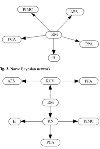
Fig. 3. Naïve Bayesian network

Fig. 4. Hierarchical Bayesian network

Table 1. List of variables used on both network models

Variable # of classes

Blood Pressure (PPA) 3

Abdominal circumference (PCA) 2

Weekly Physical Activity (AFS) 3

Body Mass Index (PIMC) 5

Parent’s Body Mass Index (H) 3

Cardiac Risk (RCV) 3

Nutritional Risk (RN) 3

Metabolic Risk (RM) 3

• Adjusting for class examples with threshold values.

• Resubmit the data set to the naïve and hierarchical networks

2.2. Modeling of Bayesian Network

In the creation of networks, cardiovascular risk and nutritional risk variables were not part of the naïve network, since they are intermediate nodes in the Bayesian network. The other variables in the naïve network are connected directly to the output node (Fig. 3).

In the hierarchical Bayesian network all variables listed are part of the network (Fig. 4).

Based on the estimated probabilities in accordance with relative frequencies, the domain expert has made an adjustment in the probability distributions of each variable. According to medical knowledge regarding the diagnosis of metabolic risk for children and adolescents, this adjustment was necessary due to a shortage of examples in the training sample and that both networks would adequately reflect the relation between variables.

2.3. Methods

In the second stage of testing, values obtained in the χ² test and by the mutual information function have been used once more in order to classify the test data set. On a first moment, the values of mutual information between dependent variables have been calculated, according to graphical models of both networks. The resulting values were used to adjust the interference of each variable in the classification. Equation (8) presents a new formula for calculating probabilities of the naïve network, as the work of Lee et al. (2011):

w (i) ij

c C a_ij d

d=arg max_∈ ∝P(c)II _∈P(a | c) (8)

Which:

d = Complete set of variables of a given test C = Output class

aij = j-th value of the i-th variable

w = Variable weight (mutual information) α = Normalization constant

and in in hierarchical network calculation is done according to the new formula, introduced by this work, as can be seen in Equation (9):

w w

i i j j j j i

P(C | A, B)=∝P(C )

∑

Which:

C = Output node A,B = Child nodes D = Intermediate node i = i-th output class

j = j-th class of intermediate value w = Variable weight (mutual information) α = Normalization constant

2.4. Data

Hospital, at Federal University of Santa Catarina, Brazil, from November 2010 to November 2011. Variables selected for the creation of networks are related to anthropometric data of physical activity, blood pressure and patient nutritional status assessment.

The sample consisted of 120 children and adolescents aged 5 to 17 years. Data collection complied with the guidelines for research involving human participants, established by Resolution No. 196/96 of the National Health Council (Brazil) (Mayer, 2012). About 100 cases were used to estimate a priori probabilities and other 20 cases for testing. Table 1 lists the variables used in Bayesian networks.

All variables are measured on an ordinal qualitative level, that is, their classes are ranked among them.

When utilizing the χ2 test it is recommended that the minimum value of expected frequency is greater or equal to five (Filho, 2008). This criterion is not satisfied in the data set used, on the variables of Weekly Physical Activity (AFS), Blood Pressure (PPA) and Parent Rating Anthropometric (H) for naïve network variables and Weekly Physical Activity (AFS) and Blood Pressure (PPA) for the hierarchical network. Thus, this recommendation was disregarded for this study.

3. RESULTS AND DISCUSSION

In order to display the summary of test results, the method known as confusion matrix (or classification matrix) has been chosen. The method is in essence quite simple, consisting primarily of a square matrix that contains all possible classes, both in rows and in columns. The matrix columns receive response values generated by the network and lines receive the output class values according to gold standard (Marsland, 2009).

Validation of Bayesian networks was performed by comparing diagnoses made by specialist physicians (gold standard) with the results of probabilities presented by both networks.

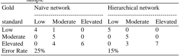
Table 2 presents test results for a sample of 20 patients, in which node classification classes are labeled “Low”, “Moderate” and “Elevated”.

On the naïve network, five cases had different classification from that provided by the specialist. On the hierarchical network, three cases have shown divergence. The remaining cases have been correctly classified.

When analyzing possible reasons that have contributed to differences between the classifications provided by the network and the gold standard, it was noted that:

• On the naïve network, in 4 out of 5 disagreeing cases, the values in one of the variables were rather close to the upper class threshold value (assuming the value of the upper class, examples came to be correctly classified)

• On the hierarchical network, the three cases in which misclassifications occurred also had threshold values

Thus, it was possible to observe that in cases where there is presence of threshold values in the input nodes, the classification obtained by Bayesian networks is affected, causing divergence in relation to the classification performed through gold standard.

This issue is present when there are nodes present that represent ordinal qualitative variables. In this situation, the class division criterion is a factor that also affects the response generated by networks.

After submitting sample data to testing both networks, the χ² test was calculated (see values for naïve and hierarchical networks in Table 3 and 4, respectively) adopting a significance level of 5% used to obtain χ²C on the chi-squared distribution table and also mutual information function values (Table 5 and 6 for naïve and hierarchical networks, respectively). The indicators generated by these metrics have been used in the analysis of dependence relations among variables.

Table 2. Classification matrix (confusion matrix) for the 20-patients

sample

Gold Naïve network Hierarchical network

--- --- standard Low Moderate Elevated Low Moderate Elevated

Low 4 1 0 5 0 0

Moderate 0 5 0 0 5 0

Elevated 0 4 6 0 3 7

Error Rate 25% 15%

Table 3. Values of χ2 for the naïve network

Naïve network-χ2 (5% significance level)

---

Statistics PIMC PCA H PPA AFS

χ2

58,61 44,49 15,82 12,53 6,77

χ2C 15,51 5,99 9,49 9,49 9,49

Table 4. Values of χ2 for the hierarchical network Hierarchical network - χ2

(5% significance level) --- Statistics RCV RN PIMC PCA H PPA AFS

χ2

18,24 71,04 130,24 61,59 23,77 116,18 28,75

The χ² test was used on a variable selection process, to verify if any variable should be disregarded in the calculation of probabilities. The mutual information function was used to weight the calculation of a

posteriori probability.

3.1. Naïve Network

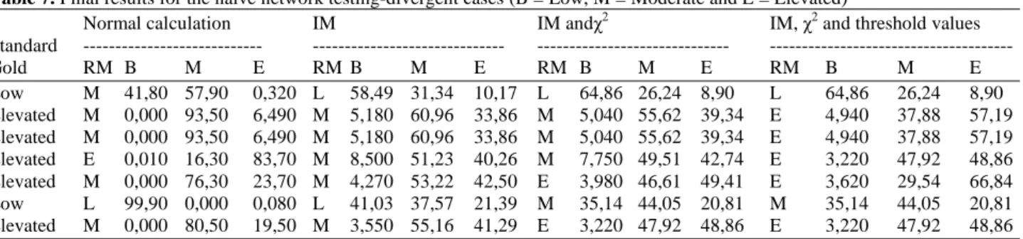
After applying the new test on the naïve network, utilizing mutual information function values, 4 cases have continued to present divergent classes. One of the cases that had been classified correctly in the first test started presenting error and one error on the first test was correctly classified. In the next step, χ² test results were used in order to eliminate network variables through a variable selection process. According to the χ² test results, the variable AFS is independent of the variable RM according to the naïve network model. In order to use this information, the AFS variable was disregarded in calculations. As a result, 2 cases have ceased presenting error and another case that had been correctly classified in the previous test, was now classified incorrectly.

After adjusting threshold data in test cases and using both calculation approaches, value of mutual information

function and variable selection through the χ² test, only one case remained with erroneous classification. By examining the data in more detail, it is possible to notice that the likely issue with this case is that the weight assigned to the PCA variable when using mutual information function, because in this example, this is the only column with a value which contributes to the output class indicated by the network. Test results with the naïve network are listed on Table 7.

Table 5. Mutual Information function values for the naïve network

Mutual information-naïve network

---

IM PIMC PCA H PPA AFS Total

Value 33,05 41,64 35,30 20,54 9,15 139,66 % 23,66 29,81 25,27 14,70 6,55 100,00

Table 6. Mutual Information function values for the hierarchical network

Mutual information-hierarchical network

---

IM RCV RN PIMC PCA H PPA AFS Total

Value 28,60 38,77 36,54 41,29 35,67 18,78 0,04 199,69 % 14,32 19,42 18,30 20,68 17,86 9,41 0,02 100,00

Table 7. Final results for the naïve network testing-divergent cases (B = Low, M = Moderate and E = Elevated)

Normal calculation IM IM andχ2 IM, χ2 and threshold values

Standard --- --- --- ---

Gold RM B M E RM B M E RM B M E RM B M E

Low M 41,80 57,90 0,320 L 58,49 31,34 10,17 L 64,86 26,24 8,90 L 64,86 26,24 8,90 Elevated M 0,000 93,50 6,490 M 5,180 60,96 33,86 M 5,040 55,62 39,34 E 4,940 37,88 57,19 Elevated M 0,000 93,50 6,490 M 5,180 60,96 33,86 M 5,040 55,62 39,34 E 4,940 37,88 57,19 Elevated E 0,010 16,30 83,70 M 8,500 51,23 40,26 M 7,750 49,51 42,74 E 3,220 47,92 48,86 Elevated M 0,000 76,30 23,70 M 4,270 53,22 42,50 E 3,980 46,61 49,41 E 3,620 29,54 66,84 Low L 99,90 0,000 0,080 L 41,03 37,57 21,39 M 35,14 44,05 20,81 M 35,14 44,05 20,81 Elevated M 0,000 80,50 19,50 M 3,550 55,16 41,29 E 3,220 47,92 48,86 E 3,220 47,92 48,86

Table 8. Final results for the hierarchical network testing-divergent cases (B = Low, M = Moderate and E = Elevated)

Normal calculation IM IM, χ2

and threshold values

Gold --- --- ---

standard RM B M E RM B M E RM B M E

Elevated M 8,77 58,70 32,60 M 0,22 0,41 0,36 E 0,21 0,31 0,47

Elevated M 8,77 58,70 32,60 M 0,22 0,41 0,36 E 0,21 0,31 0,47

Elevated M 3,59 49,10 47,30 El 0,21 0,38 0,41 E 0,14 0,33 0,52

Table 9. Classification matrix (confusion matrix) for the 20-patients sample, after adjustments

Naïve network Hierarchical network

Gold --- ---

standard Low Moderate Elevated Low Moderate Elevated

Low 4 1 0 5 0 0

Moderate 0 5 0 0 5 0

Elevated 0 0 10 0 0 10

3.2. Hierarchical Network

On the second test, while using values generated by the mutual information function performed in the hierarchical network (Table 8), 2 cases have continued to present divergent classes. When adjusting threshold values, all cases have been correctly classified. On this test, weights generated by the mutual information function have been applied only on the leaf variables, that is, nodes NB and RCV did not have their probabilities altered, since weights had already been applied to the children variables of these nodes.

In the case of the hierarchical network, the χ² test did not suggest eliminating variables, which explains the absence of the last column in Table 8.

3.3. Final Results

The final results for testing both networks can be seen in Table 9, which shows the classification matrix and where there is clear reduction in the error rate for the classification process in both networks.

4. CONCLUSION

This study presents an analysis of Bayesian classifiers, specifically hierarchical Bayesian networks and naïve Bayesian networks for a small data set (100 cases used for training and 20 for testing). To that sense, 2 networks were created, one for each model. A set of test data was submitted to each of these networks and results were recorded. In sequence, the χ² test was used to check the dependence among variables of the model in order to verify whether any of these variables should be disregarded. Then, mutual information values have been calculated to verify the amount of information that each variable carries in relation to the variable class. Furthermore, variable class intervals were analyzed in order to check threshold values which could interfere with the final classification.

The size of the data set had a strong influence in the classification process, mainly affecting the performance of the χ² test (expected frequencies below the recommended values for the test). It is suggested that the methods described herein are also applicable to larger data sets in order to eliminate the negative influence related to the amount of training examples.

The use of values generated by the mutual information function could correct errors in some classifications by attributing higher weights in the

probability calculation for certain variables. Nevertheless, one of the cases in the test was incorrectly classified due to the weight of a single variable. All other variable values in the example favored the correct class, but the elevated weight assigned to variable PIMC altered the output class to an incorrect value. In future research, this aspect will require revision.

In order to automate the task of adjusting classes of examples with threshold data, the use of fuzzy logic (Zadeh, 1965) is suggested to allow more flexibility in treating class division within model variables.

Thus, it is clear that the real gain of this study is related to improving the classification process, that is, the reduction in error rates. In the naïve Bayesian network the error rate dropped from 25% to 5%, considering the initial results of the classification process. In the hierarchical network, there was not only a 15% reduction in error rate, but it has also come to zero. Therefore, it is considered that, with the implementation of the proposed changes, there was considerable improvement in the classification process.

5. REFERENCES

Barbetta, P.A., M.M. Reis and A.C. Bornia, 2004. Estatística: Para Cursos de Engenharia e Informática. 2nd Edn., Atlas, São Paulo, ISBN-10: 8522437653, pp:410.

Cheng, J. and R. Greiner, 1999. Comparing Bayesian network classifiers. Proceedings of the 15th International Conference on Uncertainty in Artificial Intelligence, (AI’ 99),Morgan Kaufmann, pp: 101-108.

Darwiche, A., 2009. Modeling and reasoning with Bayesian networks. 1st Edn., Cambridge University Press,Cambridge,ISBN-10: 0521884381, pp:562. Filho, P.J.D.F., 2008. Introdução à Modelagem e

Simulação de Sistemas: Com Aplicações Arena. 2nd Edn., Visual Books, Florianópolis, SC, ISBN-10: 8575022288, pp:372.

Friedman, N., D. Geiger and M. Goldszmidt, 1997. Bayesian network classifiers. Mach. Learn., 29: 131-163.

Lee, C., F. Gutierrez and D. Dou, 2011. Calculating feature weights in naive bayes with Kullback-Leibler measure. Proceedings of the IEEE 11th International Conference on Data Mining, Dec. 11-14, IEEE Xplore Press, Vancouver, BC, pp: 1146-1151. DOI:10.1109/ICDM.2011.29

Marsland, S., 2009. Machine Learning: An Algorithmic Perspective. 1st Edn., CRC Press, ISBN-10: 1420067192, pp:406.

Mayer, H.C., 2012. Validação de uma Base de Conhecimento para um Sistema Especialista Bayesiano de Apoio ao Diagnóstico do Risco Metabólico. Universidade Federal de Santa Catarina.

Pearl, J., 1988. Probabilistic Reasoning in Intelligent Systems:Networks of Plausible Inference. 1st Edn., Morgan Kaufmann, San Mateo, Calif., ISBN-10: 1558604790, pp: 552.

Rish, I., 2001. An empirical study of the naïve Bayes classifier. T.J. Watson Research Center.

Russel, S. and P. Norvig, 2009. Inteligência Artificial. Elsevier.

Zadeh, L.A., 1965. Fuzzy sets. Inform. Control, 8: 338-353. Zhang, H., 2004. The optimality of naive bayes.