www.nonlin-processes-geophys.net/21/9/2014/ doi:10.5194/npg-21-9-2014
© Author(s) 2014. CC Attribution 3.0 License.
Nonlinear Processes
in Geophysics
Estimation of permeability of a sandstone reservoir by a fractal and
Monte Carlo simulation approach: a case study
U. Vadapalli, R. P. Srivastava, N. Vedanti, and V. P. Dimri CSIR-National Geophysical Research Institute, Hyderabad, India Correspondence to:N. Vedanti ([email protected])
Received: 22 April 2013 – Revised: 22 April 2013 – Accepted: 12 November 2013 – Published: 3 January 2014
Abstract.Permeability of a hydrocarbon reservoir is usually estimated from core samples in the laboratory or from well test data provided by the industry. However, such data is very sparse and as such it takes longer to generate that. Thus, esti-mation of permeability directly from available porosity logs could be an alternative and far easier approach. In this pa-per, a method of permeability estimation is proposed for a sandstone reservoir, which considers fractal behavior of pore size distribution and tortuosity of capillary pathways to per-form Monte Carlo simulations. In this method, we consider a reservoir to be a mono-dispersed medium to avoid effects of micro-porosity. The method is applied to porosity logs obtained from Ankleshwar oil field, situated in the Cambay basin, India, to calculate permeability distribution in a well. Computed permeability values are in good agreement with the observed permeability obtained from well test data. We also studied variation of permeability with different parame-ters such as tortuosity fractal dimension (Dt), grain size (r) and minimum particle size (d0), and found that permeability is highly dependent upon the grain size. This method will be extremely useful for permeability estimation, if the average grain size of the reservoir rock is known.
1 Introduction
Permeability is one of the important parameters that govern production of hydrocarbons from reservoirs. As we know, fluid flow in reservoirs depends upon permeability, and in the case of multiple phases of hydrocarbons, it is relative permeability that governs the fluid flow. Estimation of the permeability of a geological medium is a difficult job, as it varies over several orders of magnitude, even for a sin-gle rock such as sandstone (Clauser, 1992; Nelson, 1994;
and Li (2001) deduced a unified model for describing the fractal character of porous media and proposed a criterion to determine whether a porous medium can be characterized by fractal theory and technique or not. An analytical expression for the permeability of a fractal bi-dispersed porous medium was developed by Yu and Cheng (2002). However, if a porous medium is a multiscale or scale-dependent fractal medium, analytical expression may not give accurate results. To over-come this issue, Yu et al. (2005) proposed the Monte Carlo technique to simulate the permeability of fractal porous me-dia. Yu and Li (2004) derived analytical expressions of the fractal dimensions for wetting and non-wetting phases for unsaturated porous media. Liu and Yu (2007) established a fractal relative permeability model that takes into account the capillary pressure difference effect in the case of unsaturated porous media. Yu (2008) reviewed the theories and achieve-ments in the field of application of fractal geometry to un-derstand flow in porous media. Xu and Yu (2008) derived an expression for the Kozeny–Carman constant by using the an-alytical formula of permeability. The Monte Carlo simulation technique is used by Xu et al. (2012) to estimate relative per-meability. A fractal model for capillary pressure is obtained by Xiao and Chen (2013). Xu et al. (2013a) used fractal the-ory and the Monte Carlo simulation technique to develop a probability model for radial flow in fractured porous media. Analytical expressions for relative permeabilities of wetting and non-wetting phases are presented by Xu et al. (2013b). The innovative work presented by Yu et al. (2005) assumed a model in which a porous medium consists of a set/bundle of parallel and tortuous capillaries with uniform diameter and obtained probability model for pore diameter and permeabil-ity. The probability model comprehends the fractal nature of pore size distribution and tortuous capillaries. The overall ap-proach consists of simulating random pore size distribution to calculate flow rate from the Hagen–Poiseuille equation (Denn, 1980) and then, by using Darcy’s law (Darcy, 1856), an expression for permeability is obtained. This fractal-based method was applied to estimate the permeability of a sintered copper bi-dispersed porous medium to solve a heat transport problem (Yu et al., 2005).
The estimation of the permeability of a hydrocarbon reser-voir is one of the important goals of reserreser-voir geophysicists. In the present work, a fractal-based Monte Carlo simulation approach is applied for the first time to estimate the perme-ability of the Ankleshwar sandstone hydrocarbon reservoir, situated in the Cambay basin, India. The reservoir formation consists mainly of alternate layers of sandstone and shale. As we know that sandstones and shales are porous fractal me-dia (Katz and Thomson, 1985; Krohn and Thompson, 1986; Krohn, 1988b; Sahimi, 2011), we performed Monte Carlo simulations based on the fractal nature of pore size distri-bution in porous media of the reservoir. We assumed the reservoir as a mono-dispersed porous medium to study the effect of macro-porosity on permeability. A mono-dispersed porous medium considers only macro-pores formed between
the grains and ignores micro-pores inside the clusters, which do not contribute towards macro-porosity.
1.1 Fractal description of pore structures
A porous medium consists of tortuous capillary pathways. The tortuous length of these capillary pathways follows the fractal/scaling law. The scaling relationship for capillary length in heterogeneous porous media is given byLt(ε)=
ε1−DtLDt
0 , whereε,LtandL0are the scale of measurement, tortuous length and characteristic (straight) length, respec-tively andDtis the tortuosity fractal dimension (Wheatcraft and Tyler, 1988). Yu and Cheng (2002) considered pore di-ameter (λ)as the scale of measurement. Thus, the smaller the diameter, the longer the capillary and scaling law that can be given as
Lt(λ)=λ1−DtLD0t, (1) where 1< Dt<2, representing the extent of convolutedness of capillary pathways for fluid flow through a medium. The higher the value ofDt, the more the convolutedness or
tortu-osity. The limiting values ofDt=1 andDt=2 correspond respectively to a straight capillary and a highly tortuous line that fills a plane (Wheatcraft and Tyler, 1988).
A porous medium consists of a large number of pores of varying pore diameters that intersect the pore cross sections. The size distribution of pore diameters is another important property. This distribution is analogous to cumulative size distribution of islands on the Earth’s surface, which follows the fractal scaling law (Mandelbrot, 1982; Majumdar and Bhushan, 1990). Pitchumani and Ramakrishnan (1999) and Yu and Cheng (2002) have established a fractal scaling law to describe the distribution of pores in a porous medium, which is given as:
N (L≥λ)=
λ max
λ
Df
, (2)
whereN is the number of pores with diameter (L) greater than or equal toλ,Dfthe pore area dimension, with 1< Df< 2, representing the fractal dimension of the intersecting pore cross sections with a plane normal to the flow direction. It is evident from Eq. (2) that whenλapproaches maximum pore
size,λmax, the number of pores greater than or equal toλmax is one. Conversely, when λapproaches smallest pore size, λmin, the numbers of pores are maximum, and the scaling law becomes
Nt(L≥λmin)= λ
max
λmin Df
, (3)
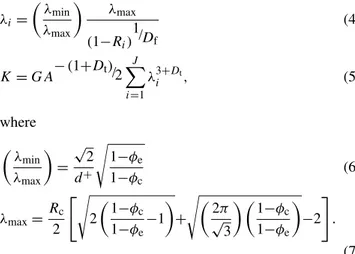
Based on these fractal scaling laws, Yu et al. (2005) ob-tained probability expressions for pore diameter and perme-ability in terms of pore diameter as given below:
λi= λ
min
λmax
λ
max
(1−Ri)1/Df
(4)
K=GA−(1+Dt)/2
J X
i=1
λ3i+Dt, (5)
where λ
min
λmax
= √
2
d+ s
1−φe
1−φc (6)
λmax=Rc 2
"s 2
1 −φc 1−φe−1
+
s 2π
√ 3
1−φc 1−φe
−2
#
.
(7) In the case of a bi-dispersed porous medium, effective porosity is given by Yu and Cheng (2002) as below.
φe=
A−π R2c/2
+φcπ Rc2/2
A , (8)
where φe=effective porosity, φc=micro-porosity inside cluster,Rc=cluster mean radius,d+=ratio of cluster mean diameter to the minimum particle size (d0), λi=diameter
of the ith capillary tube chosen by the Monte Carlo sim-ulation, A=total cross-sectional area of a unit cell, and
G=geometry factor for flow through a circular capillary.
In a bi-dispersed porous medium, small particles form clusters. The spaces between clusters form macro-pores and within the cluster micro-pores exist.
2 Geology of Ankleshwar oil field, Cambay basin
Ankleshwar oil field lies in the western part of the Cambay basin, India (Fig. 1). The field is doubly plunging anticline, trending ENE–WSW. It has a multi-layered sandstone reser-voir of deltaic origin. Ankleshwar formation, which was de-posited during the marine regression phase during the Up-per to Middle Eocene (Holloway et al., 2007) is the major stratigraphic unit in the field. The formation consists of four sub-lithological units, viz., Telwa shale (effective seal), Ar-dol, Kanwa shale and Hazad members from top to bottom (Fig. 5). A Hazad member is an important reservoir sand-stone; however, it contains shale laminae. The Ardol section comprises sand-shale alterations. The Ankleshwar formation is overlain by the Dadhar formation and underlain by Cam-bay shale, which is the source rock.
Fig. 1.Location of the Cambay basin and its oil and gas fields (after www.spgindia.org/paper/sopt_2313/tmp_2313). Ankleshwar field is highlighted by the ellipse in the figure.
Table 1.Gamma ray values adopted to discriminate pure sand, pure shale and shaly sand.
lithology Gamma ray value (API)
pure sand <˙35 pure shale >65
shaly sand ≥35 or≤65
3 Methodology
3.1 Estimation of porosity from density log
Porosity is derived from density log using the following equation:
φ=ρb−ρm ρf−ρm
, (9)
whereρb=bulk density of the formation, ρm=density of the rock matrix, ρf=density of the fluids occupying the porosity, andφ=porosity of the rock.
Table 2.Estimated permeability (K) for a range of porosities and for different values of grain radius (r), minimum particle size (d0), tortuosity fractal dimension (Dt)and pore area fractal dimension (Df).
S.NO. r(mm) d0(µm) Dt Df
K(mD)
porosity (%)
15 20 25 30
1 0.1 1 1.8 1.7 233 312 368 412 2 0.05 1 1.8 1.65 90 210 260 301 3 0.05 2 1.8 1.58 119 265 345 375 4 0.05 1 1.6 1.65 130 257 312 351
Thus, to discriminate between pure sand, pure shale and shaly-sand intervals in the well, the criteria shown in Table 1 were adopted. We know that shale is more porous than sand-stone, but pores are not interconnected, and hence cannot per-meate fluid. Hence, to find effective or interconnected poros-ity of shaly-sand intervals, bulk densporos-ity (ρb)is corrected for shale volume using Eq. (10), which is given as:
(ρb)corr=(ρb)clean(1−Vsh)+(ρb)shaleVsh, (10) where(ρb)corr=corrected bulk density of the shaly lithol-ogy,(ρb)clean=bulk density of clean sand stone formation,
(ρb)shale=bulk density of pure shale, andVsh=shale vol-ume, which is calculated from the gamma-ray log using the Dresser tertiary equation.
The values of (ρb)clean and (ρb)shale are 2.19 g cm−3 and 2.36 g cm−3, respectively, which are selected from depth in-tervals 1150 m to 1158 m and 1184 m to 1194 m, respectively, in the log. The corrected value of density is then used in Eq. (9) to obtain effective porosity of shaly-sand intervals, which is given as:
φe=
(ρb)corr−ρm
ρf−ρm . (11)
In shaly-sand intervals clay minerals occupy pores or they cover the sand grains, thereby forming micro-pores and in-troducing micro-porosity (φc), which is the porosity below which there is no permeating flow (the percolation threshold) (Nabovati et al., 2009). In such cases, in place of effective porosity, useful porosity (φuse) (http://www.spec2000.net) can be used, which is given as:
φuse=φe−φc (12)
φc=φe×C, (13)
whereC is a constant that can be obtained from shale vol-ume, as shown below:
C= Vsh
(Vsh+Vsand) (14)
Vsand=1−(Vsh+φe). (15)
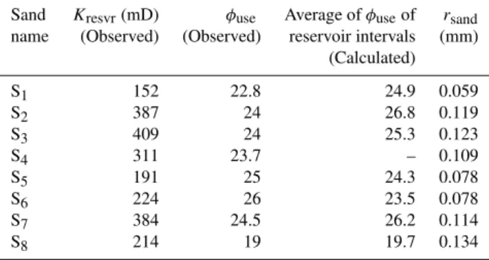
Table 3.The observed average useful porosity, observed average reservoir permeability (kresvr), calculated average useful porosity of reservoir intervals and estimated grain radius for different sand layers in the formation.
Sand Kresvr(mD) φuse Average ofφuseof rsand
name (Observed) (Observed) reservoir intervals (mm) (Calculated)
S1 152 22.8 24.9 0.059
S2 387 24 26.8 0.119
S3 409 24 25.3 0.123
S4 311 23.7 – 0.109
S5 191 25 24.3 0.078
S6 224 26 23.5 0.078
S7 384 24.5 26.2 0.114
S8 214 19 19.7 0.134
Here, we assume that permeability estimation by using useful porosity is a more efficient way, as in this case the con-tribution of micro-porosity to permeability becomes negligi-ble. In the present work, a well W1 drilled in the Ankleshwar sandstone reservoir cutting across the Telwa, Ardol, Kanwa, Hazad and Cambay lithological units is used for the analysis. The Hazad and Ardol sections of the reservoir are divided into eight sand layers, which are named S1 to S8. Intervals of these sand layers with useful porosity greater than 15 % are considered as reservoir intervals. The average useful poros-ity obtained from the reservoir intervals for each sand layer is given in Table 3. The calculated useful porosity of differ-ent sand layers matches with the information given by the operator in this well.
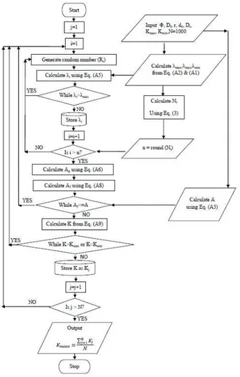
3.2 Monte Carlo simulations for prediction of permeability
Monte Carlo simulation is a random search method, widely used in geophysics, using generation of random numbers (Dimri, 1992). The method allows the generation of many possible models. In the present work, the method suggested by Yu et al. (2005) is applied to the Ankleshwar sandstone reservoir, where micro-pores are formed by pore-filling ma-terial (clays) or exist as intra-granular pores (Krohn, 1988a). The permeability contribution by these micro-pores is neg-ligible (Yu and Lee, 2000; Nimmo, 2004; Loucks, 2005). Hence, as discussed above, it is more appropriate to run the simulations with macro-porosity or φuse. After removal of micro-porosity, clusters become solid grains; hence instead of cluster mean radius, grain radius (r) can be used. In this case Eq. (8) becomes:
φuse= A−π r 2/2
A . (16)
Fig. 2.Flow chart to apply the Monte Carlo simulation technique for permeability estimation.
3.3 Variation of permeability with tortuosity fractal dimension (Dt), and average grain radius (r) and minimum particle size (d0)
Monte Carlo simulations are run for different values of grain radius, tortuosity fractal dimension and minimum particle size to understand permeability variation with these parame-ters. The mean value of increment in permeability for a small variation in grain radius from 0.05 mm to 0.1 mm is 38 %, as shown in Fig. 3a (whenDt=1.8 and d0=1 µm). Simi-larly, whenDt=1.8 andr=0.05 mm, the minimum particle size (d0)is increased from 1 µm to 2 µm, then permeability is increased by 22 %, as shown in Fig. 3b. Next, whenDt is increased from 1.6 to 1.8 by consideringd0=1 µm and
r=0.05 mm, permeability is reduced by 20 %, as shown in Fig. 3c. In each caseDfis calculated from Eq. (A4). The es-timated permeability for different values ofr,Dt,d0andDf is given in Table 2. This analysis suggests that permeability is more sensitive to change in grain radius thanDtandd0.
(a)
(b)
(c)
Fig. 3. (a),(b)and(c), respectively shows permeability variations with grain radius (r), minimum particle size (d0)and tortuosity frac-tal dimension (Dt). Permeability decreases with an increase inDt
Table 4.Average values of reservoir permeability in each layer estimated for different values ofDtandd0and from the Kozeny–Carman equation. For each estimated set the RMS error with respect to observed average reservoir permeability is given.
Calculated permeability (K) in mD
RMS error w.r.t. Observed
Sand name S1 S2 S3 S5 S6 S7 S8
Dt=1.75 andd0=1 µm 276 405 404 288 272 388 322 74.6
Dt=1.75 andd0=1.5 µm 297 435 440 313 292 420 351 95.5
Dt=1.75 andd0=2 µm 326 479 482 342 320 459 406 130.1
Dt=1.8 andd0=1 µm 248 367 365 261 243 354 294 58.7
Dt=1.8 andd0=1.5 µm 267 395 398 281 262 382 326 71.2
Dt=1.8 andd0=2 µm 301 437 441 314 293 422 357 98.2
Dt=1.85 andd0=1 µm 238 357 359 250 234 345 278 53.4
Dt=1.85 andd0=1.5 µm 259 384 389 271 256 368 324 67.2
Dt=1.85 andd0=2 µm 292 425 429 303 285 414 352 90.6
Dt=1.87 andd0=1 µm 240 355 354 247 231 340 274 54.13
Dt=1.87 andd0=1.5 µm 259 378 383 271 254 362 304 63.3
Dt=1.87 andd0=2 µm 284 417 429 297 277 406 343 84.4
Kozeny–Carman equation 123 430 152 167 648 546 113 119.6
Fig. 4. Permeability versus porosity plot for well (W1). Calcu-lated average reservoir permeability (circles) falls in the range of observed average reservoir permeability values (stars). Sand layer names (S1 to S8) annotated to the data points clearly show the amount of deviation from predicted permeability with respect to the corresponding observed value.
3.4 Estimation of grain radius
Sand grains in different reservoir layers can have different radii. Mavko and Nur (1997) incorporated micro-porosity into the Kozeny–Carman equation, which we used to com-pute the distinct grain radius of reservoir layers and the equa-tion is given below:
r=p72τ2K(1+φc−φe) (φe−φc)
3 2
. (17)
Equation (17) is based on the assumption that formation is made up of spherical grains of uniform diameter.
However, we have assumed that the observed average reservoir permeability and average porosity pairs as shown in Table 3, available from well test data, are those of pure sandstone layers because the reservoir consists of a negligi-ble amount of shale. In this caseφcis zero,φeis equal toφuse and thus in this case grain radius,rwill becomersand, which is the radius of sand grains and can be given as
rsand= p
72τ2Kresvr(1−φuse)
(φuse)3/2
, (18)
whereKresvris the observed average reservoir permeability. In Eq. (18) tortuosity (τ )is unknown. The average grain radius of theS1andS3layers measured from core samples in nearby wells is 0.069 mm and 0.142 mm, respectively (R. Sharma, personal communication, 2012). Thus, using known grain radii, the average value ofτ is estimated as 6.99. For
other sand layers (S2, S4 to S8), rsand is estimated from Eq. (18) and the values are given in Table 3. However, in case of shaly-sand intervals, the effective grain radius (reff)
is calculated using a weighted average formula using volume fractions as the weights, which is given as
reff=
d0
2
Vsh+(rsand)Vsand
Vsh+Vsand
. (19)
3.5 Assigning the values to tortuosity fractal dimension (Dt) and minimum particle size (d0)
In order to select the values of Dt andd0, simulations are run for several values (1.75, 1.8, 1.85 and 1.87) of Dt and three different values (1.0 µm, 1.5 µm, 2.0 µm) of d0, with
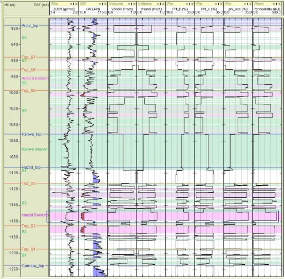
Fig. 5.Well logs of well (W1). Pure sandstone (<35 API) and shale (>65 API) are colored in red and blue on the gamma ray curve, respectively. Pink color bars and green color bars represent pure sandstone and shaly sand (≥35 API or≤65 API), respectively. The zone highlighted by rectangles corresponds to a pure sandstone interval in the S3 layer that shows the highest permeability (409 mD), which matches with the observed value.
litholog given by the operator shows the presence of clay in all the formations, we assumed minimum particle size (d0) of clay grade, which are defined as the grains with 1 to 2 µm diameters. As we know that permeability decreases with an increase inDt(Fig. 3c) and observed reservoir permeability values are low, we chose higher values ofDt for the analy-sis. For all possible pairs ofDt andd0,, permeability of all
the sand layers is calculated. In each sand layer the average of useful porosity and permeability over all the reservoir in-tervals (Table 4) is calculated and compared with the cor-responding observed average porosity and average reservoir permeability available from well tests (Table 3).
Root mean square error (RMSE) between calculated and observed values is measured for each pair ofDtandd0.
4 Results and discussions
The calculated average reservoir permeability of each sand layer for all the pairs ofDt andd0 and the corresponding RMS error are given in Table 4. It is clear from Table 4 that
Dt=1.85 andd0=1 µm give the least value of the RMS er-ror, which is 53.4 mD. The mean value of Df for all sand layers, calculated from Eq. (A4), is 1.67. The RMS error between observed and calculated porosity is 1.8 %. Perme-ability of all sand layers is also calculated from the Kozeny– Carman equation (Eq. 17) by replacingφe−φcwithφuseand “r” withreff. In this case the RMS error between calculated and observed values is 119.6 mD (Table 4).
shale, effective porosity, critical porosity, useful porosity and permeability are shown in Fig. 5. The highest value of per-meability (409 mD) is obtained for reservoir zone S3, which is highlighted by rectangles in Fig. 5. This value exactly matches with the observed permeability of the S3 layer ob-tained from well test data. For the S4 sand layer, the calcu-lated value of permeability (27 mD) is very close to the ob-served non-reservoir permeability (23 mD) provided by the operator.
The permeability of each sand layer in the Ankleshwar formation is estimated with the confirmed set of fractal di-mensions, minimum particle size and estimated grain radius. Figure 4 clearly shows that, for most of the sand layers, the error between calculated and observed permeability does not exceed 50 mD, except in the case of the S1 sand layer, where the error is 86 mD. As we know, permeability obtained from well test data corresponds to a larger area in reservoir; how-ever, permeability obtained by logs represents a smaller area around the well. This may also result in a mismatch between observed and calculated permeabilities. Another reason for the difference between observed and calculated permeabili-ties can be grain size, which is a very important parameter.
Since most of the evaluated permeability values match with the corresponding observed values within acceptable error range, the estimated values ofDt andd0are reliable. From Fig. 5 it is obvious that porosity and permeability logs clearly discriminate pure sand, shaly sand and shale intervals, with higher values for pure sand, lower values for shaly sand and lowest values for shale. In the present well, S4 sand hav-ing very low permeability (27 mD) is non-reservoir, which is because of silt stone present in this interval (according to the litholog given by the operator). The Kanwa interval is de-fined as shale according to general geology; however, in the present well, according to the litholog given by the operator, a small amount of sandstone present in this interval reduces gamma-ray readings and thus this interval is shaly sand. It is obvious from the RMS error values given in Table 4 that Monte Carlo simulations give better results than the Kozeny– Carman equation.
Thus, by considering a mono-dispersed porous medium and modifying the method given by Yu et al. (2005), we could develop a methodology for estimation of reservoir per-meability without using any empirical constant. The flow chart of the modified algorithm is also presented.
5 Conclusions
We found that accurate permeability estimation requires a good control of grain radius. In the major pay zone of the reservoir, the calculated permeability value (409 mD) exactly matches with the observed permeability value provided by the operator. In other sand layers, the difference between calculated and observed average reservoir permeability is ±50 mD, which is acceptable in this case.
Thus, in the absence of well test data or laboratory mea-surements, this method can be used to obtain first-hand in-formation on reservoir permeability. Using this method, we can obtain continuous permeability distribution in reservoirs if porosity distribution from seismic data is known.
Appendix A
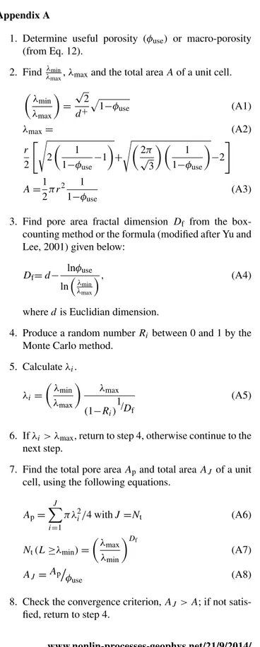
1. Determine useful porosity (φuse) or macro-porosity (from Eq. 12).
2. Find λmin
λmax,λmaxand the total areaAof a unit cell.
λ min λmax = √ 2 d+ p
1−φuse (A1)
λmax= (A2)
r
2 "s
2 1
1−φuse−1 + s 2π √ 3 1 1−φuse
−2
#
A=1
2π r 2 1
1−φuse (A3)
3. Find pore area fractal dimension Df from the box-counting method or the formula (modified after Yu and Lee, 2001) given below:
Df=d− lnφuse lnλmin
λmax
, (A4)
wheredis Euclidian dimension.
4. Produce a random numberRi between 0 and 1 by the
Monte Carlo method. 5. Calculateλi.
λi = λ
min
λmax
λ
max
(1−Ri)1/Df
(A5)
6. Ifλi> λmax, return to step 4, otherwise continue to the next step.
7. Find the total pore areaApand total areaAJ of a unit
cell, using the following equations.
Ap= J X
i=1
π λ2i/4 withJ=Nt (A6)
Nt(L≥λmin)= λ
max
λmin Df
(A7)
AJ =Apφuse (A8)
8. Check the convergence criterion,AJ> A; if not
9. Whenever convergence criterion is satisfied, calcu-late the permeability K (withDt measured from the box-counting method or using the method given in Sect. 3.5).
K=GA−(1+Dt)/2
J X
i=1
λ3i+Dt (A9)
10. Repeat the procedure for N number of times (say
N=1000) to getN values of permeability and take
the mean to compute the final value of permeability. 11. Check the criterion,Kmin< K < Kmax, if not satisfied
return to step 4 (where,KminandKmaxare acceptable minimum and maximum reservoir permeabilities re-spectively).
Acknowledgements. We acknowledge the Royal Norwegian
Embassy, New Delhi for providing financial support through the Indo-Norwegian research project. We thank the Director of IRS, Ahmedabad and Ankleshwar asset for providing some of the information. We thank the Director, NGRI for his kind support to carry out this work. One of the authors (VPD) is grateful to the Director General, CSIR, New Delhi for awarding a distinguished scientist project. We are thankful to O. P. Pandey, Kirti Srivastava and all other group members for their useful suggestions and encouragement. One of the authors (U. Vadapalli) is thankful to CSIR for providing a research internship.
Edited by: L. Telesca
Reviewed by: two anonymous referees
References
Adler, P. M. and Thovert, J. F.: Fractal porous media, Transport in porous media, 13, 41–78, 1993.
Carman, P. C.: Flow of gases through porous media, Butterworth Scientific Publications, 1956.
Clauser, C.: Permeability of crystalline rocks, EOS, 73, 233–238, 1992.
Darcy, H.: Les Fontaines Publiques de la Ville de Dijon, Dalmont, Paris, 1856.
Denn, M. M.: Process Fluid Mechanics, Prentice-Hall, Englewood Cliff, NJ, 35–66 pp., 1980.
Dimri, V. P.: Deconvolution and Inverse Theory: Application to Geophysical Problems, Elsevier Science Ltd., 71 pp., 1992. Dimri, V. P. (Ed.): Fractal Dimensional analysis of soil for flow
studies, in: Application of fractals in Earth Sciences, Balkema, USA/Oxford and IBH publishing Co. Pvt. LTD., 189 – 193, 2000a.
Dimri, V. P.: Application of fractals in Earth Sciences, Balkema, USA/Oxford and IBH publishing Co. Pvt. LTD., 2000b. Dimri, V. P. (Ed.): Fractal behavior of the Earth System, Springer,
New York, 2005.
Dimri, V. P., Vedanti, N., and Chattopadhyay, S.: Fractal analysis of aftershock sequence of the Bhuj earthquake: A wavelet-based approach, Current Sci., 88, 1617–1620, 2005.
Dimri, V. P., Srivastava, R. P., and Vedanti, N.: Fractal models in ex-ploration geophysics: application to hydrocarbon reservoirs, El-sevier, Amsterdam, 2012.
Feranie, S. and Latief, F. D. E.: Tortuosity–porosity relationship in two-dimensional fractal model of porous media, Fractals, 21, 1350013, doi:10.1142/50218348*13500138, 2013.
Holloway, S., Garg, A., Kapshe, M., Pracha, A. S., Khan, S. R., Mahmood, M. A., Singh, T. N., Kirk, K. L., Applequist, L. R., Deshpande, A., Evans, D. J., Garg, Y., Vincent, C. J., and Williams, J. D. O.: A regional assessment of the potential for CO2storage in the Indian subcontinent, Sustainable and
Renew-able Energy Programme Commissioned Report CR/07/198 by British Geological Survey (BGS), NERC, 2007.
Katz, A. J. and Thompson, A. H.: Fractal sandstone pores: Implica-tions for conductivity and pore formation, Phys. Rev. Lett., 54, 1325–1328, 1985.
Kozeny, J.: Über die kapillare Leitung des Wassersim Boden (Auf-stiegVersickerung und Anwendeung auf die Bewässerung), Sitz. Ber, Akad. Wiss.Wien, math. Nat (Abt. IIa), 136a, 271–306, 1927.
Krohn, C. E.: Sandstone Fractal and Euclidean Pore Volume Distri-butions, J. Geophysi. Res., 93, 3286–3296, 1988a.
Krohn, C. E.: Fractal measurements of sandstones, shales and car-bonates, J. Geophys. Res., 93, 3297–3305, 1988b.
Krohn, C. E. and Thompson, A. H.: Fractal sandstone pores: Au-tomated measurements using scanning-electron-microscope im-ages, Phys. Rev. B, 33, 6366–6374, 1986.
Liu, Y. and Yu, B. M.: A fractal model for relative permeability of unsaturated porous media with capillary pressure effect, Fractals, 15, 217–222, 2007.
Loucks, R. G.: Revisiting the Importance of Secondary Dissolution Pores in Tertiary Sandstones along the Texas Gulf Coast, Gulf Coast Association of Geological Societies Transactions, 55, 448– 455, 2005.
Mandelbrot, B. B.: Fractal geometry of nature, W.H. Freeman, New York, 23–57, 1982.
Majumdar, A. and Bhushan, B.: Role of fractal geometry in rough-ness characterization and contact, J. Tribology, 112, 205–216, 1990.
Mavko, G. and Nur, A.: The effect of a percolation threshold in the Kozeny–Carman relation, Geophysics, 62, 1480–1482, 1997. Nabovati, A., Llewellin, E. W., and Sousa, A. C. M.: A general
model for the permeability of fibrous porous media based on fluid flow simulations using the lattice Boltzmann method, Compos-ites, 40, 860–869, 2009.
Nelson, P. H.: Permeability – porosity relationships in sedimentary rocks, log Analyst, 35, 38–62, 1994.
Nimmo, J. R.: Porosity and Pore Size Distribution, Encyclopedia of Soils in the Environment, 3, 295–303, 2004.
Pape, H., Clauser, C., and Iffland, J.: Permeability prediction based on fractal pore-space geometry, Geophysics, 64, 1447–1460, 1999.
Pitchumani, R. and Ramakrishnan, B.: fractal geometry model for evaluating permeabilities of porous preforms used in liquid com-posite molding, Int. J. Heat Mass Transfer, 42, 2219–2232, 1999. Sahimi, M.: Flow and Transport in Porous Media and Fractured
Rock: From Classical Methods to Modern Approaches, 2011. Sahimi, M. and Yortsos, Y. C.: Applications of fractal geometry to
Smidt, J. M. and Monro, D. M.: Fractal modeling applied to reser-voir characterization and flow simulation, Fractals, 6, 401–408, 1998.
Srivastava, R. P. and Sen, M.: Stochastic inversion of prestack seismic data using fractal-based initial models, Geophysics, 75, R47–R59, 2010.
Sub surface understanding of an Oil field in Cambay basin, available at: http://www.spgindia.org/paper/sopt_2313/tmp_2313, last ac-cess: 3 June 2013.
Vedanti, N. and Dimri, V. P.: Fractal behavior of electrical properties in oceanic and continental crust, Indian J. Geo-Marine Sci., 32, 273–278, 2003.
Vedanti, N., Srivastava, R. P., Pandey, O. P., and Dimri, V. P.: Frac-tal behavior in continenFrac-tal crusFrac-tal heat production, Nonlin. Pro-cesses Geophys., 18, 119–124, doi:10.5194/npg-18-119-2011, 2011.
Wheatcraft, S. W. and Tyler, S. W.: An explanation of scale de-pendent dispersivity in heterogeneous aquifers using concepts of fractal geometry, Water Resour. Res., 24, 566–578, 1988. Xiao, B. and Chen, L.: A Fractal Model for Capillary Pressure of
Porous Media, Research Journal of Applied Sciences, Engineer-ing and Technology, 6, 593–597, 2013.
Xu, P. and Yu, B. M.: Developing a new form of permeability and Kozeny – Carman constant for homogeneous porous media by means of fractal geometry, Adv. Water Res., 31, 74–81, 2008. Xu, P., Yu, M. Z., Qiu, S. X., and Yu, B. M.: Monte–Carlo
simula-tion of a two-phase flow in an unsaturated porous media, Thermal Science, 16, 1382–1385, 2012.
Xu, P., Yu, B. M., Qiao, X., Qiu, S., and Jiang, Z.: Radial perme-ability of fractured porous media by Monte–Carlo simulations, International Journal of Heat and Mass transfer, 57, 369–374, 2013a.
Xu, P., Qiu, S., Yu, B. M., and Jiang, Z.: Prediction of relative per-meability in unsaturated porous media with a fractal approach, Int. J. Heat Mass Transfer, 64, 829–837, 2013b.
Young, I. M. and Crawford, J. W.: The fractal structure of soil ag-gregations: its measurement and interpretation, J. Soil Sci., 42, 187–192, 1991.
Yu, B. M.: Analysis of flow in fractal porous media, Appl. Mech. Rev., 61, 050801, doi:10.1115/1.2955849, 2008.
Yu, B. M. and Cheng, P.: A fractal permeability model for bi-dispersed porous media, Int. J. Heat Mass Transfer, 45, 2983– 2993, 2002.
Yu, B. M. and Lee, L. J.: A simplified in-plane permeability model for textile fabrics, Polymer Composites, 21, 660–685, 2000. Yu, B. M. and Li, J.: Some fractal characters of porous media,
Frac-tals, 9, 365–372, 2001.
Yu, B. M. and Li, J.: Fractal dimensions for unsaturated porous me-dia, Fractals, 12, 17–22, 2004.