Universidade Federal de Minas Gerais
Programa de P´os-Graduac¸˜ao em Engenharia El´etrica Escola de Engenharia
Techniques for Controlling Swarms of Robots
Luciano Cunha de Ara´
ujo Pimenta
Thesis presented to the Graduate Program in Electrical Engineering of the Federal University of Minas Gerais in partial fulfillment of the requirements for the degree of Doctor in Electrical Engineering.
Advisor: Prof. Renato Cardoso Mesquita
Co-Advisor: Prof. Guilherme Augusto Silva Pereira Foreign Advisor: Prof. Vijay Kumar
Universidade Federal de Minas Gerais
Programa de P´os-Graduac¸˜ao em Engenharia El´etrica Escola de Engenharia
T´
ecnicas para o Controle de Enxames de
Robˆ
os
Luciano Cunha de Ara´
ujo Pimenta
Tese apresentada ao Curso de P´os-Gradua¸c˜ao em Enge-nharia El´etrica da Universidade Federal de Minas Gerais como requisito parcial para obten¸c˜ao do t´ıtulo de Doutor em Engenharia El´etrica.
Orientador: Prof. Renato Cardoso Mesquita
Co-orientador: Prof. Guilherme Augusto Silva Pereira Orientador Estrangeiro: Prof. Vijay Kumar
To my love, Carina.
Abstract
This thesis addresses the problem of controlling very large groups of robots, refereed as swarms. Scalable solutions in which there is no need for labelling the robots are proposed. All the robots run the same software and the success of the task execution does not depend on specific members of the group. Robustness to dynamic addition and deletion of agents is also an advantage of our approaches. In the first methodology, we model the swarm as a fluid immersed in a region where a field of external forces, which is free of local minima, is defined. In this case, the Smoothed Particle Hydrodynamics (SPH) method is applied to model the “robotic fluid”, more specifically, to model the interactions among the robots of the group. The Finite Element Method (FEM) is also used in this work to compute the fields that determine external forces. This approach is instantiated in a pattern generation task and also in a coverage task. In the second methodology, a problem of opti-mal environment coverage using robots equipped with sensors is addressed by means of tools from the Locational Optimization theory. Three important extensions of well-known results in the literature are presented: (i) sensors with different footprints, (ii) disk-shaped robots, and (iii) nonconvex polyg-onal environments. Both approaches are verified in simulations. The first technique is also implemented and tested in actual robots.
Resumo
Esta tese aborda o problema de controle de grandes grupos de robˆos, referidos como enxames. S˜ao propostas solu¸c˜oes escal´aveis as quais n˜ao ne-cessitam da identifica¸c˜ao ´unica dos robˆos. Todos os robˆos executam o mesmo c´odigo e o sucesso na execu¸c˜ao de uma tarefa n˜ao depende de membros es-pec´ıficos do grupo. Robustez `a adi¸c˜ao e remo¸c˜ao dinˆamica de agentes tamb´em ´e uma vantagem das abordagens propostas. Na primeira metodologia, o en-xame ´e modelado como um fluido imerso numa regi˜ao onde um campo de for¸cas externas livre de m´ınimos locais ´e definido. Neste caso, utiliza-se o m´etodo de Hidrodinˆamica de Part´ıculas Suavizadas (HPS) para modelar o “fluido rob´otico”, mais especificamente, para modelar as intera¸c˜oes entre robˆos do grupo. O M´etodo de Elementos Finitos (MEF) tamb´em ´e utili-zado neste trabalho para calcular os campos vetoriais que determinam as for¸cas externas. Esta abordagem ´e instanciada num problema de gera¸c˜ao de padr˜oes e tamb´em num problema de cobertura de ambientes. Na segunda metodologia, um problema de cobertura ´otima de ambientes utilizando robˆos equipados com sensores ´e tratado por meio de ferramentas provenientes da teoria de Otimiza¸c˜ao Locacional. S˜ao apresentadas trˆes extens˜oes impor-tantes de resultados j´a conhecidos na literatura: (i) sensores com diferentes campos de vis˜ao, (ii) robˆos com formato circular e (iii) ambientes poligo-nais n˜ao-convexos. Ambas metodologias s˜ao verificadas em simula¸c˜oes. A primeira metodologia ´e tamb´em implementada e testada em robˆos reais.
Acknowledgments
I would like to thank first my wife, Carina, for her love, support, compre-hension, and for always be with me. I would like to thank my whole family, specially my father, my mother, my brother, and my grandmother for their love, support, and for everything they have done for me. I am also very grateful to Carina’s family for the great friendship and for always receiving me with happiness.
Thanks to Professor Renato Cardoso Mesquita and Professor Guilherme Augusto Silva Pereira who were fundamental in this work. Thanks for the shared knowledge , the excellent orientation, the trustiness, the friendship and for the doors that were opened.
Thanks also to Professor Vijay Kumar, who was also essential in the development of this work, for the great opportunities that he offered me and for the excellent orientation during the time I worked in his lab, GRASP, at the University of Pennsylvania.
I am grateful to the students of GOPAC, Miguel, L´eo Corrˆea, and Ju-liano for their help with the computational implementations and for their friendship. I am grateful to all members of GOPAC, specially to my friends Alexandre, Ricardo, Carrano, Douglas, and Mozelli for creating an excellent work environment. Thanks also to the remaining friends of GEP, VER-LAB, and CPDEE for their friendship. Many thanks to the colleagues at the GRASP Lab for the shared knowledge, specially to Nathan Michael and
ACKNOWLEDGMENTS v
Quentin Lindsey for the help with experiments.
Many thanks to the members of my thesis committee, professors Fernando Cesar Lizarralde, Geovany Ara´ujo Borges, Marco Henrique Terra, Leonardo Antˆonio Borges Tˆorres, Luiz Chaimowicz, and Elson Jos´e da Silva for their valuable suggestions.
Thanks to professors M´ario Campos, Hani, Walmir, Paulo Seixas, Marcos Severo, Porf´ırio, Pedro Donoso, and Jaime for the shared knowledge and for always be available to help when I needed. Thanks also to the remaining professors that somehow were essential in my academic formation.
Agradecimentos
Gostaria de agradecer primeiramente `a minha esposa, Carina, pelo amor, apoio, compreens˜ao e por sempre estar ao meu lado. Gostaria de agradecer `a toda a minha fam´ılia, especialmente ao meu pai, `a minha m˜ae, ao meu irm˜ao e `a minha av´o pelo amor, apoio e por tudo que fizeram por mim. Sou muito grato tamb´em `a fam´ılia da Carina pela grande amizade e por sempre me receberem com alegria.
Agrade¸co ao Professor Renato Cardoso Mesquita e Professor Guilherme Augusto Silva Pereira os quais foram essenciais na realiza¸c˜ao deste trabalho. Agrade¸co pelo conhecimento compartilhado, pela excelente orienta¸c˜ao, pela confia¸ca, pela amizade e pelas portas que me foram abertas.
Agrade¸co tamb´em ao Professor Vijay Kumar, o qual foi tamb´em essen-cial no desenvolvimento deste trabalho, pelas grandes oportunidades que ele me proporcionou e pela excelente orienta¸c˜ao durante o doutorado sandu´ıche realizado em seu laborat´orio, GRASP, na Universidade da Pensilvˆania.
Sou grato aos alunos do GOPAC, Miguel, L´eo Corrˆea e Juliano pelo grande apoio nas implementa¸c˜oes computacionais e pela amizade. Sou grato aos demais membros do GOPAC, especialmente aos amigos Alexandre, Ri-cardo, Carrano, Douglas e Mozelli por proporcionarem um ´otimo ambiente de trabalho. Agrade¸co tamb´em aos demais amigos do GEP, do VERLAB e do CPDEE pelo grande companheirismo. Agrade¸co tamb´em aos colegas do GRASP Lab pela troca de conhecimentos, especialmente Nathan Michael e
AGRADECIMENTOS vii
Quentin Lindsey pela ajuda na realiza¸c˜ao de experimentos.
Gostaria tamb´em de agradecer aos membros da minha banca, professores Fernando Cesar Lizarralde, Geovany Ara´ujo Borges, Marco Henrique Terra, Leonardo Antˆonio Borges Tˆorres, Luiz Chaimowicz e Elson Jos´e da Silva pelas valiosas sugest˜oes.
Muito obrigado aos professores M´ario Campos, Hani, Walmir, Paulo Sei-xas, Marcos Severo, Porf´ırio, Pedro Donoso e Jaime pelo conhecimento ensi-nado e por estarem sempre dispon´ıveis quando precisei. Agrade¸co tamb´em aos demais professores que foram fundamentais na minha forma¸c˜ao.
Resumo Estendido
Introdu¸c˜
ao
A Rob´otica cooperativa ´e o campo da rob´otica dedicado ao estudo de t´ecnicas que permitem que robˆos em um time cooperem entre si e com seres humanos para realizar uma dada tarefa. Para uma grande variedade de tarefas, sistemas rob´oticos cooperativos fornecem solu¸c˜oes que n˜ao podem ser obtidas utilizando um ´unico robˆo. Al´em disso, mesmo em situa¸c˜oes onde um ´unico robˆo possa ser utilizado, o uso de um time pode ter custo mais baixo, ser mais confi´avel, ser mais tolerante a falhas e ainda mais flex´ıvel.
Controlar grupos de robˆos tem sido um desafio e diferentes solu¸c˜oes j´a foram propostas. O tamanho do grupo ´e um fator crucial que determina o tipo mais apropriado de abordagem. Basicamente, existem duas categorias de abordagens: centralizadas e descentralizadas. As abordagens centraliza-das s˜ao aquelas que assumem a existˆencia de uma entidade central, a qual ´e capaz de planejar as a¸c˜oes de cada robˆo do grupo. Embora, em geral, se possa provar que a utiliza¸c˜ao de tal abordagem garante sucesso na realiza¸c˜ao da tarefa, este tipo de t´ecnica n˜ao ´e escal´avel para grandes grupos de robˆos por raz˜ao de limita¸c˜oes computacionais. Por outro lado, abordagens descen-tralizadas fornecem solu¸c˜oes escal´aveis uma vez que neste caso cada agente do grupo planeja suas pr´oprias a¸c˜oes baseadas em informa¸c˜oes locais.
Em acordo com as id´eias de solu¸c˜oes escal´aveis, um novo paradigma
ix
chamado enxame de agentes autˆonomos tem sido estudado no campo da rob´otica. Neste paradigma o objetivo ´e controlar grandes grupos de robˆos (dezenas a centenas) muito simples. A id´eia chave ´e que o sucesso na execu¸c˜ao de uma tarefa depender´a dos comportamentos que v˜ao emergir das intera¸c˜oes entre agentes. Neste contexto, cada agente deve ser o mais simples poss´ıvel com capacidades limitadas de comunica¸c˜ao, sensoreamento e atua¸c˜ao. Outra caracter´ıstica importante de um enxame ´e a flexibilidade. Utilizando dife-rentes mecanismos de coordena¸c˜ao o mesmo enxame pode ser utilizado em diferentes problemas. Um outro ponto importante ´e que a coordena¸c˜ao do en-xame n˜ao deve depender de membros espec´ıficos do grupo. Logo, solu¸c˜oes to-talmente descentralizadas, onde os agentes podem ser considerados anˆonimos e podem ser programados com o mesmo c´odigo, devem ser consideradas. Al´em disso, tais solu¸c˜oes devem ser robustas `a adi¸c˜ao e remo¸c˜ao dinˆamica de robˆos.
x
Contribui¸c˜
oes
Este trabalho contribuiu para a ´area de enxames rob´oticos com novas t´ecnicas escal´aveis para a coordena¸c˜ao de enxames. As contribui¸c˜oes princi-pais s˜ao:
• Controladores descentralizados por meio do acoplamento entre dois m´etodos num´ericos: a Hidrodinˆamica de Part´ıculas Suavizadas (HPS) e o M´etodo de Elementos Finitos (MEF). Os controladores propostos dependem apenas de informa¸c˜oes locais. Al´em disso, todos os robˆos podem ser considerados entidades anˆonimas. Um tratamento eficiente de obst´aculos tamb´em ´e parte da metodologia proposta.
• Uma solu¸c˜ao para o problema de gera¸c˜ao de padr˜oes utilizando mo-delo de fluido incompress´ıvel. O enxame ´e modelado como um fluido incompress´ıvel sujeito a for¸cas externas. Como os robˆos s˜ao controlados afim de manter a densidade do fluido constante, esta abordagem possibilita uma maneira indireta de controlar fra-camente a conectividade do grupo. Problemas relacionados `a im-plementa¸c˜ao em robˆos reais como o tamanho do robˆo e ainda res-tri¸c˜oes n˜ao-holonˆomicas s˜ao abordados. Garantias de desvio de obst´aculos s˜ao discutidas. Na ausˆencia de obst´aculos, apresentam-se pela primeira vez provas de estabilidade e convergˆencia de controla-dores baseados em HPS. [Pimenta et al., 2006b, Pimenta et al., 2006c, Pimenta et al., 2007a, Pimenta et al., 2008b]
xi
• Trˆes novas e importantes extens˜oes de uma abordagem para cober-tura ´otima utilizando redes de sensores m´oveis [Cortez et al., 2004]: (i) incorpora¸c˜ao de heterogeneidade no time de robˆos permitindo que diferentes tipos de sensores sejam utilizados. Utiliza-se o chamado
Power diagram [Aurenhammer, 1987] para definir a regi˜ao de do-minˆancia de cada agente; (ii) solu¸c˜ao das limita¸c˜oes pr´aticas relati-vas `a considera¸c˜ao de robˆos pontuais por meio da introdu¸c˜ao de um problema de minimiza¸c˜ao com restri¸c˜oes; e (iii) generaliza¸c˜ao para ambientes n˜ao-convexos com a introdu¸c˜ao de diagramas de Voronoi geod´esicos [Aronov, 1989] na lei de controle. [Pimenta et al., 2008a]
Coordena¸c˜
ao de Enxames Utilizando Modelos
de Dinˆ
amica dos Fluidos
xii
Isto se deve `a habilidade de tal m´etodo no uso de malhas n˜ao-estruturadas. Controladores descentralizados s˜ao derivados a partir de um acoplamento entre a HPS e o MEF.
A HPS ´e uma t´ecnica sem malhas, Lagrangiana, baseada em part´ıculas. As equa¸c˜oes da HPS s˜ao derivadas a partir das equa¸c˜oes governantes cont´ınuas por meio de uma interpola¸c˜ao a partir de um conjunto desorde-nado de part´ıculas. Em problemas de dinˆamica dos fluidos, cada part´ıcula representa um pequeno volume do fluido e a interpola¸c˜ao ´e realizada pelo uso de fun¸c˜oes n´ucleo, W, diferenci´aveis que aproximam uma fun¸c˜ao delta. Neste trabalho utilizam-se splinesc´ubicas:
W(r, h) = 10
7πh2
1−3 2κ
2+3 4κ
3 se 0≤κ≤1, 1
4(2−κ)
3 se 1≤κ≤2,
0 caso contr´ario,
(1)
ondeκ=krk/h. Pode-se observar que o suporte desta fun¸c˜ao ´e dado por 2h. As equa¸c˜oes governantes cont´ınuas s˜ao convertidas num conjunto de equa¸c˜oes diferenciais ordin´arias, onde cada uma controla a evolu¸c˜ao de um atributo de uma part´ıcula espec´ıfica. As equa¸c˜oes governantes de dinˆamica dos fluidos s˜ao trˆes: (i) conserva¸c˜ao da massa; (ii) conserva¸c˜ao do momento; e (iii) conserva¸c˜ao da energia. Para fluidos compress´ıveis na ausˆencia de fluxo de calor, as equa¸c˜oes de conserva¸c˜ao correspondentes da HPS para a part´ıcula i s˜ao:
ρi =
X
j
mjW(qi−qj, h), (2)
dvi
dt =−
X j mj µ Pi ρ2 i
+Pj
ρ2
j
+ Πij
xiii dei dt = 1 2 X j mj µ Pi ρ2 i
+Pj
ρ2
j
+ Πij
vij · ∇iWij, (4)
onde ρ ´e densidade, v ´e velocidade, P ´e press˜ao, e ´e energia interna por unidade de massa,Wij =W(qi−qj) ´e a fun¸c˜ao n´ucleo,vij =vi−vj efi ´e a
soma das for¸cas externas normalizadas pela massami. O termo Πij ´e o termo
de viscosidade artificial incorporado para tratar choques. Existem diversas variantes para este termo e a mais utilizada ´e dada por [Monaghan, 1992]:
Πij =
1
ρij(−ξ1cijµij+ξ2µ
2
ij) if vij ·qij <0,
0 if vij ·qij >0,
(5)
onde
µij =
hvij ·qij
kqijk2+η2
. (6)
Em (5), ρij ´e a m´edia entre as densidades das part´ıculas ie j,ξ1 eξ2 s˜ao
constantes de viscosidade, cij ´e a m´edia das velocidades do som e η2 ´e um
termo para evitar singularidades.
Para a modelagem de fluidos incompress´ıveis considera-se a seguinte equa¸c˜ao de estado [Monaghan, 1994]:
Pi =Bi
·µ ρi ρ0 ¶γ −1 ¸ , (7)
onde ρ0 ´e a densidade de referˆencia e Bi ´e o chamado m´odulo Bulk. Este
m´odulo est´a relacionado `a compressibilidade do fluido. Com a utiliza¸c˜ao de (7), o sistema ´e for¸cado a regular sua densidade para a densidade de referˆencia.
descen-xiv
tralizados no sentido de que apenas informa¸c˜ao local ´e necess´aria: o campo externo na posi¸c˜ao do robˆo e posi¸c˜oes e velocidades de robˆos vizinhos. Para um robˆo i com configura¸c˜ao qi = [xi, yi]T, os robˆos vizinhos s˜ao definidos
como aqueles no conjunto de vizinhan¸ca Ni:
Ni ={j 6=i|kqj−qik< D}, (8)
onde a distˆanciaD´e determinada pelo tamanho do suporte da fun¸c˜ao n´ucleo. Primeiramente, assume-se tamb´em que os robˆos s˜ao pontuais e ho-lonˆomicos com modelo dado por:
¨
qi =ui(q,q˙, t), (9)
onde q= [qT
1, . . . ,qTN]T ´e a configura¸c˜ao do grupo.
O primeiro problema tratado ´e o problema de gera¸c˜ao de padr˜oes geom´etricos bidimensionais:
Problem 0.1 Seja um grupo de N robˆos com distribui¸c˜ao espacial inicial qualquer, o ambiente com obst´aculos est´aticos definindo um dom´ınio com-pactoΩ⊂R2 e uma curvaΓ :I →Ω, onde I ⊂R. Encontre um controlador
que guie os robˆos para formar o padr˜ao descrito por Γ sem colidir uns com os outros e sem colidir com os obst´aculos est´aticos.
Para resolver tal problema prop˜oe-se o controlador:
ui(q,q˙) =bi−ζvi+kfi, (10)
onde
bi =−
X
j
mj
µ
Pi
ρ2
i
+ Pj
ρ2
j
+ Πij
xv
k eζ s˜ao constantes positivas de ajuste e fi ´e determinado a partir do vetor
−∇φ. A fun¸c˜ao φ´e uma fun¸c˜ao potencial que garante convergˆencia das cur-vas intergrais de−∇φpara o padr˜ao desejado. Em ambientes com obst´aculos utilizam-se fun¸c˜oes harmˆonicas calculadas por meio do M´etodo de Elementos Finitos. O problema de valor de contorno a ser resolvido ´e dado por:
∇2φ= 0,
φ(Γ1) = φ(Γ2) = 0,
φ(∂Ω1) = φ(∂Ω2) =φ(P) = Vc,
(12)
onde φ ´e a fun¸c˜ao harmˆonica, Vc ´e uma constante positiva, e P ´e um ponto
definido no interior do padr˜ao para o caso de curvas fechadas. As curvas Γ1 e
Γ2 definem as fronteiras de uma regi˜ao tal que Γ est´a em seu interior. Al´em
disso, ∂Ω1 define as fronteiras externas do dom´ınio e∂Ω2 define as fronteiras
dos obst´aculos.
Para ambientes sem obst´aculos podem-se utilizar as shape functions. Es-tas fun¸c˜oes s˜ao fun¸c˜oes positivas semi-definidas com valor m´ınimo igual a zero sobre a curva desejada. S˜ao obtidas provas de estabilidade e convergˆencia utilizando-se tais fun¸c˜oes.
O segundo problema tratado ´e um problema de cobertura restrita:
Problem 0.2 Encontre controladores descentralizados que guiem uma rede
de sensores m´oveis para uma configura¸c˜ao final que maximiza a cobertura sensorial total e mant´em a densidade maior ou igual a um valor de referˆencia
ρ0.
xvi
Problemas relacionados `a implementa¸c˜ao da t´ecnica proposta em robˆos reais tamb´em s˜ao tratados. O fato dos robˆos reais n˜ao serem pontuais ´e tratado por meio de uma adapta¸c˜ao da viscosidade artificial, uma vez que este termo garante termos repulsivos que evitam colis˜oes entre part´ıculas. A adapta¸c˜ao ´e dada por:
µij =
hvij ·qij
(kqijk −(2R+ε))2
, (13)
onde R ´e o raio do robˆo e ε´e um fator de seguran¸ca.
Restri¸c˜oes n˜ao-holonˆomicas tamb´em s˜ao tratadas. Mais especifica-mente, consideram-se as restri¸c˜oes a que est˜ao sujeitos robˆos diferenciais. Neste caso, utiliza-se a t´ecnica de lineariza¸c˜ao por realimenta¸c˜ao de esta-dos [Murray et al., 1994]:
v
ω
=
cos(θ) sin(θ) −sin(dθ)
cos(θ)
d
·
˙
xd
˙
yd
, (14)
onde v ´e a velocidade linear, ω ´e a velocidade angular e d ´e a distˆancia do ponto de referˆencia da lineariza¸c˜ao ao centro do robˆo. O vetor de entrada [ ˙xd,y˙d]T corresponde `as velocidades desejadas.
Utiliza-se ainda neste trabalho uma estrat´egia de part´ıculas virtuais. Es-tas part´ıculas s˜ao colocadas exatamente sobre a fronteira dos obst´aculos. Tais part´ıculas s˜ao utilizadas para garantir que n˜ao existam colis˜oes entre robˆos e obst´aculos, uma vez que as for¸cas externas podem ser insuficientes para evitar tais colis˜oes.
xvii
pr´oximas do mundo real. Os experimentos foram realizados utilizando-se a infra-estrutura do GRASP (General Robotics, Automation, Sensing, and Perception) Lab na Universidade da Pensilvˆania, Estados Unidos. Esta infra-estrutura conta com robˆos Scarabs e um sistema de cˆameras no teto que permite localizar cada robˆo no ch˜ao durante o experimento. Detalhes desta infra-estrutura podem ser encontrados em [Michael et al., 2008].
Cobertura ´
Otima de Ambientes Baseada em
Otimiza¸c˜
ao Locacional
Uma abordagem distribu´ıda e ass´ıncrona para cobertura sensorial ´otima de uma regi˜ao convexa utilizando agentes sensores m´oveis idˆenticos pontuais ´e proposta em [Cortez et al., 2004]. Cada agente (robˆo) segue uma lei de controle baseada em gradiente descendente que tem o objetivo de minimizar um funcional que codifica a qualidade da cobertura sensorial. Esta lei de controle depende apenas de informa¸c˜oes de posi¸c˜oes dos robˆos e dos seus vizinhos imediatos. Neste contexto, vizinhos s˜ao definidos como os robˆos localizados em c´elulas de Voronoi vizinhas. O funcional tamb´em utiliza uma fun¸c˜ao densidade que determina pesos para pontos ou ´areas do ambiente que s˜ao mais importantes que outras. Assim, ´areas com altos valores de fun¸c˜ao densidade devem ser melhor cobertas que ´areas com baixos valores.
Seja uma representa¸c˜ao do ambiente Ω ⊂ RN. Seja tamb´em P =
{q1, . . . ,qn} a configura¸c˜ao de n sensores m´oveis, onde qi ⊂ Ω.
Consi-dere a parti¸c˜ao T = {T1, . . . , Tn} tal que I(Ti)∩I(Tj) = ∅, ∀i 6= j, onde I(·) representa o interior de uma dada regi˜ao e ∪n
i=1Ti = Ω. A id´eia chave ´e
xviii
cobertura que mede o desempenho do sistema ´e definido por:
H(P, T) =
n
X
i=1
H(qi, Ti) = n
X
i=1
Z
Ti
f(d(q,qi))ϕ(q)dq, (15)
onde d corresponde a uma fun¸c˜ao que mede distˆancias entre pontos q ∈ Ω e sensores. A fun¸c˜ao ϕ : Ω → R+ ´e a fun¸c˜ao densidade. Esta fun¸c˜ao reflete
um conhecimento da probabilidade de ocorrˆencia de eventos em diferentes regi˜oes, ou simplesmente uma medida de importˆancia relativa de diferentes regi˜oes de Ω. A fun¸c˜aof :R→R´e uma fun¸c˜ao suave estritamente crescente
sobre a imagem de d, que mede a degrada¸c˜ao do desempenho de sensores com a distˆancia. O problema de cobertura do ambiente, Ω, ´e traduzido para o problema de minimiza¸c˜ao do funcional em (15).
Primeiramente, prova-se que uma condi¸c˜ao necess´aria para um m´ınimo do funcional em (15) ´e que a parti¸c˜ao T deve ser uma parti¸c˜ao de Voronoi,
V(P), de acordo com a fun¸c˜ao de distˆanciad. Al´em disso, prova-se a condi¸c˜ao necess´aria:
∂H(P)
∂qi
= ∂H(qi, Vi)
∂qi
=
Z
Vi
∂
∂qi
f(d(q,qi))ϕ(q)dq= 0. (16)
Dado o conjunto de pontosP ={q1, . . . ,qn}distribu´ıdos sobre o dom´ınio
Ω, com fronteira ∂Ω, a c´elula de Voronoi Vi associada ao pontoqi de acordo
com a fun¸c˜ao de distˆancia d´e definida por:
Vi ={q∈Ω|d(q,qi)≤d(q,qj),∀j 6=i}. (17)
A cole¸c˜ao de tais regi˜oes forma a chamada parti¸c˜ao de Voronoi.
Em [Cortez et al., 2004] utiliza-se distˆancia Euclidiana como d, e f(d) =
xix
que as c´elulas de Voronoi s˜ao politopos convexos. Neste caso o m´ınimo do funcional de cobertura ´e obtido quando os agentes est˜ao localizados exata-mente no centr´oide das c´elulas de Voronoi correspondentes. O centr´oide ´e dado por:
q∗i =
R
Viqϕ(q)dq
R
Viϕ(q)dq
. (18)
Considera-se o modelo cinem´atico para os agentes:
˙
qi =ui. (19)
A lei de controle proposta em [Cortez et al., 2004] ´e dada por:
ui =−k(qi−q∗i), (20)
onde k ´e um ganho positivo. Esta lei de controle ´e baseada no gradiente descendente uma vez que:
∂H
∂qi
= 2
µZ
Vi
ϕ(q)dq
(qi−q∗i).
´
E importante ressaltar que em geral o sistema converge para um m´ınimo local j´a que o funcionalH ´e n˜ao-convexo.
Nesta tese, s˜ao propostas trˆes extens˜oes para a estrat´egia em [Cortez et al., 2004]. A primeira extens˜ao considera sensores hete-rogˆeneos com campos de vis˜ao circulares com diferentes raios Rqi. O
funcional de cobertura, neste caso, ´e dado por:
H(P, P V) =
n
X
i=1
Z
P Vi
[kq−qik2−Rq2i]ϕ(q)dq, (21)
dis-xx
tance [Aurenhammer, 1987]. A parti¸c˜ao requerida neste caso ´e o chamado
power diagram,P V.
Opower diagram,P V, associa uma regi˜ao,P Vi a cada c´ırculoBi(qi, Rqi)
em R2. Tal regi˜ao ´e definida por:
P Vi ={q∈R2|d(q,qi)≤d(q,qj),∀j 6=i}, (22)
onde a power distance d(q,qi) =kq−qik2−R2qi.
A lei de controle para esta extens˜ao ´e a mesma apresentada anteriormente em (20) com a diferen¸ca de que o centr´oide agora ´e dado por:
q∗i =
R
P Viqϕ(q)dq
R
P Viϕ(q)dq
. (23)
O que ´e mais interessante na utiliza¸c˜ao dapower distance ´e que as regi˜oes de dominˆancia de cada agente ser˜ao novamente politopos convexos.
A segunda extens˜ao trata de agentes sensores n˜ao pontuais. Mais espe-cificamente, agentes circulares com raio rqi. O funcional de cobertura neste
caso ´e o mesmo utilizado em [Cortez et al., 2004], ou seja, d ´e a distˆancia Euclidiana e f(d) = d2. Define-se, primeiramente, a regi˜ao de Voronoi livre
FVi:
FVi ={q∈Vi|kq−q∂Vik ≥rqi,∀q∂Vi}, (24)
onde k · k´e a norma Euclidiana e q∂Vi ´e um ponto da fronteira da regi˜ao de
xxi
Prop˜oe-se ent˜ao a solu¸c˜ao do problema de minimiza¸c˜ao com restri¸c˜oes:
min
qi H
(P, V) (25)
s.t.
gi1(qi)≤0, . . . , gim(qi)≤0
onde gil(qi) = 0 define a l-´esima face da regi˜ao FVi. A minimiza¸c˜ao ´e
reali-zada por meio de uma lei de controle baseada num m´etodo de proje¸c˜ao de gradiente:
1. Se nenhuma restri¸c˜ao est´a ativa
ui =−k
∂H
∂qi
, (26)
2. Caso contr´ario
ui =kπ
µ
−∂H
∂qi
, ∂FVi
, (27)
onde π³−∂∂qH
i, ∂FVi
´
fornece a proje¸c˜ao do vetor −∂∂qH
i sobre o vetor til, o
qual ´e um vetor unit´ario tangente `a l-´esima face da regi˜ao FVi.
A terceira e ´ultima extens˜ao considera ambientes poligonais n˜ao-convexos. O funcional de cobertura ´e dado por:
H(P, T) =
n
X
i=1
H(qi, Ti) = n
X
i=1
Z
Ti
d(q,qi)2ϕ(q)dq, (28)
onded(q,qi) ´e o comprimento do caminho mais curto entre qeqi, ou seja, ´e
xxii
A lei de controle proposta ´e dada por:
ui =−k
∂H
∂qi
= 2k
Z
Vi
d(qi,q)ϕ(q)zqi,qdq, (29)
onde zqi,q ´e um vetor unit´ario com dire¸c˜ao do vetor suporte do primeiro
segmento do caminho mais curto entre qi e q.
Simula¸c˜oes num´ericas ideais utilizando o modelo em (19) verificam as leis de controle propostas.
Conclus˜
oes
pro-xxiii
blema de gera¸c˜ao de padr˜oes geom´etricos e tamb´em no problema de cobertura com densidade restrita. T´ecnicas para acomodar as caracter´ısticas de robˆos reais como o tamanho e as restri¸c˜oes n˜ao-holonˆomicas s˜ao propostas. Basica-mente, isto ´e atingido pelo uso da lineariza¸c˜ao por realimenta¸c˜ao de estados e tamb´em pela adapta¸c˜ao do termo de viscosidade artificial das equa¸c˜oes de fluido. O campo vetorial calculado a partir da fun¸c˜ao harmˆonica ajuda no desvio dos obst´aculos est´aticos. Entretanto, tal campo vetorial pode ser insuficiente para evitar colis˜oes. Uma estrat´egia que coloca part´ıculas vir-tuais nas fronteiras dos obst´aculos ´e proposta para garantir a ausˆencia de colis˜oes. Os termos de viscosidade artificiais associados `as part´ıculas virtu-ais s˜ao respons´aveis por garantir esta ausˆencia. Simula¸c˜oes computacionvirtu-ais ideais, simula¸c˜oes real´ısticas e experimentos utilizando robˆos reais foram exe-cutados para mostrar a efic´acia do m´etodo.
No caso de tarefas de cobertura sensorial de ambientes, uma proprie-dade muito desejada ´e otimaliproprie-dade. Entretanto, ´e dif´ıcil provar que os con-troladores propostos baseados em HPS conduzem os robˆos para uma confi-gura¸c˜ao ´otima para cobertura. Logo, foram investigadas novas ferramentas para garantir otimalidade. Neste trabalho, foram utilizadas ferramentas da otimiza¸c˜ao locacional para obter leis de controle ´otimas e distribu´ıdas. Esta estrat´egia tamb´em mant´em uma das principais funcionalidades da aborda-gem baseada em fluidos que ´e a habilidade de controlar a densidade dos robˆos sobre uma dada regi˜ao. Foram incorporadas trˆes novas extens˜oes a trabalhos encontrados na literatura [Lloyd, 1982, Cortez et al., 2004] para considerar: (i) sensores com campos de vis˜ao circulares de diferentes raios; (ii) robˆos com forma geom´etrica circular; e (iii) ambientes poligonais n˜ao-convexos. As ex-tens˜oes s˜ao baseadas no uso de diferentes fun¸c˜oes de distˆancia,power distance
xxiv
Ambas as t´ecnicas, HPS e otimiza¸c˜ao locacional, s˜ao descentralizadas uma vez que apenas informa¸c˜oes locais s˜ao requeridas. Isto ´e importante para garantir escalabilidade. Na primeira t´ecnica cada agente necessita de infoma¸c˜ao de agentes localizados dentro de um dado raio de distˆancia. Na segunda t´ecnica cada agente busca informa¸c˜oes de seus vizinhos de Voronoi.
´
Contents
List of Figures xxvii
List of Tables xxx
List of Symbols xxxi
1 Introduction 1
1.1 Motivation . . . 2 1.2 Methodology . . . 4 1.3 Contributions . . . 6 1.4 Organization . . . 8
2 Background 9
2.1 Workspace . . . 9 2.2 Configuration Space . . . 11 2.3 Motion Constraints . . . 14 2.3.1 Holonomic Mobile Robot . . . 16 2.3.2 Nonholonomic Robot . . . 17 2.4 Lyapunov Stability Theory . . . 19 2.5 Navigation Functions . . . 21 2.6 Harmonic Functions . . . 25 2.7 Finite Element Method . . . 28 2.7.1 Discretization . . . 28 2.7.2 Potential and Gradient Computation . . . 30 2.8 Smoothed Particle Hydrodynamics . . . 33 2.9 Voronoi Tessellation . . . 41
3 Related Work 43
3.1 Biologically Inspired Approaches . . . 43 3.2 Physics Based Methods . . . 45 3.3 Techniques from Mathematical Tools . . . 48
CONTENTS xxvi
4 A Fluid Based Approach for Swarm Control 51
4.1 The Pattern Generation Problem . . . 52 4.2 Pattern Generation Task Solution . . . 53 4.2.1 Global Potential Functions . . . 53 4.2.2 Controllers based on a Fluid Model . . . 57 4.2.3 Virtual Particles . . . 61 4.2.4 Analysis . . . 64 4.3 Numerical Simulations . . . 73 4.3.1 Static Obstacles - Examples . . . 74 4.3.2 Dynamic Obstacles - Examples . . . 77 4.4 Experimental Results . . . 84 4.5 Environment Coverage . . . 87
5 Coverage Control Based on Locational Optimization Tools 94
5.1 Locational Optimization Framework . . . 95 5.1.1 Centroidal Voronoi Tessellation . . . 96 5.1.2 Continuous-Time Lloyd Algorithm . . . 99 5.2 Heterogeneous Robots . . . 100 5.3 Robots with Finite Size . . . 103 5.4 Nonconvex Environments . . . 106 5.5 Simulation Results . . . 109
6 Conclusions 114
6.1 Summary . . . 114 6.2 Publications . . . 116 6.3 Future Work . . . 119
List of Figures
1.1 Experiments with real robots. (a) Four robots caging a circu-lar robot [Pereira, 2003]. (b) Distributed boundary coverage with a swarm of miniature robots [Correll, 2007]. . . 3 2.1 Typical mobile robot workspace. . . 10 2.2 A robot is represented by a point in its configuration space.
A trajectory is then a continuous sequence of configurations that starts at q0 (the initial robot’s configuration) and ends
atqd (the desired final configuration) [Pereira, 2003]. . . 12
2.3 Result of the growth of a rectangular obstacle by the size of a triangular robot with constant orientation [Pimenta, 2005]. . . 13 2.4 Nonholonomic constraint in differential drive robots. . . 18 2.5 Local minimum caused by a U-shaped obstacle. . . 23 2.6 Path followed by an actual holonomic robot under the
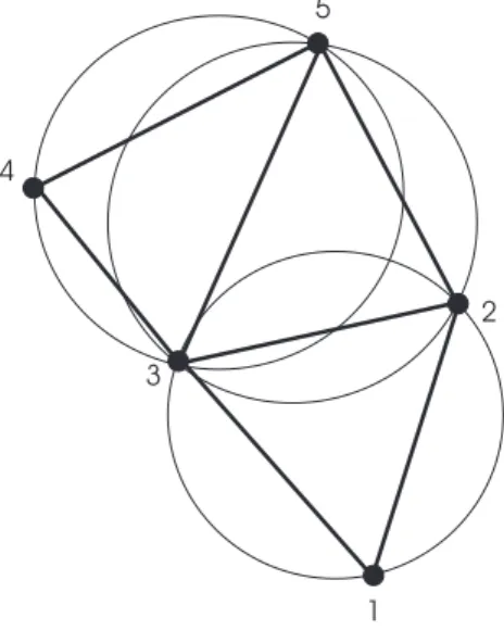
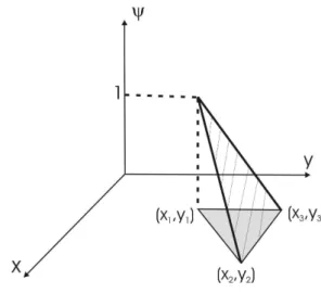
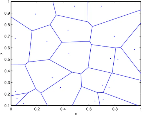
influ-ence of a discretized harmonic field [Pimenta et al., 2006a]. . . 28 2.7 Delaunay triangulation of a set of 5 points in the plane. . . 30 2.8 Linear interpolation function defined over a triangular element. 31 2.9 Graphic of the kernel function W with h= 1. . . 36 2.10 Example of a Voronoi tessellation in the case of Euclidean
distance in a 2D domain. . . 42 4.1 Domain example. . . 55 4.2 Feedback linearization point. The light grey circle represents
a circular robot with radiusR. Assuming a feedback lineariza-tion point at a distancedfrom the center, the white circle with radius R′ =R+d is used to guarantee collision avoidance. . . 61 4.3 Multiple virtual particles in an occupancy grid. (a) Robot and
obstacles. (b) Virtual particles from occupied cells. . . 62 4.4 Worst scenarios for collision avoidance. Fig. 4.4(a) worst
sce-nario for a pair of robots. Fig. 4.4(b) worst scesce-nario for a robot (grey circle) and a virtual particle (black circle). . . 71
LIST OF FIGURES xxviii
4.5 Vector field in an environment with a rectangular obstacle. . . 75 4.6 81 robots generating a circle pattern in the presence of a
rect-angular static obstacle. (a) Initial distribution. (b) Split. (c) Final distribution. . . 76 4.7 324 robots generating a star shape. (a) Start. (b) Intermediate
instant. (c) End. . . 77 4.8 Convergence to the reference density. (a) Density of one
par-ticle along all the iterations. (b) Histogram of the density of all particles along all the iterations. . . 78 4.9 Simulation with 121 point robots from a starting configuration
(a) to the goal (d), with intermediate configurations (b) and (c). . . 79 4.10 196 robots generating a circle pattern in the presence of
dy-namic particle obstacles - Part I. . . 81 4.11 196 robots generating a circle pattern in the presence of
dy-namic particle obstacles - Part II. . . 82 4.12 169 robots generating a circle pattern in the presence of a
dynamic square obstacle. The simulation was stopped before the particles generate the complete pattern. . . 83 4.13 The 20 × 13.5× 22.2 cm3 differential drive robotics platform
(a) with camera (b) without camera. . . 85 4.14 Simulation with 15 robots from a starting configuration (Fig.
4.14(a)) to the goal (Fig. 4.14(d)), with intermediate configu-rations (Figs. 4.14(b) and 4.14(c)). . . 86 4.15 Experimental Results. A team of seven robots, starting from
an initial configuration (Fig. 4.15(a)), control around an ob-stacle (Figs. 4.15(c), 4.15(e), and 4.15(g)) to a goal circu-lar formation (Fig. 4.15(i)). The results in the configuration space are also shown in Figs. 4.15(b), 4.15(d), 4.15(f), 4.15(h), and 4.15(j). . . 88 4.16 Coverage simulation result. A team of twenty robots cover a
building-like environment from a starting configuration 4.16(a) to a final configuration 4.16(h), with intermediate configura-tions 4.16(b), 4.16(c), 4.16(d), 4.16(e), 4.16(f), and 4.16(g). . 92 4.17 Density of the team over iterations. (a) Mean density. (b)
Density standard deviation. . . 93 5.1 Power cells. Fig. 5.1(a) Two disjoint circles. Fig. 5.1(b)
LIST OF FIGURES xxix
5.2 Linear constraints for a disk-robot with radiusrqi. The dotted
lines represent the facets of ∂FVi, which are given by gi1 = 0,
gi2 = 0, gi3 = 0, and gi4 = 0, with gradients as in Fig. 5.2(a).
Given the active setA ={gi1} in Fig. 5.2(b) we compute the
control inputui by projecting the negative gradient ofHonto
the unit vector ti1 which is tangent to the active facet. . . 105
5.3 Simulation results for heterogeneous agents in a environment with density function defined as in (5.30). In the panels on the left, the large circle with diameter 0.6 units represents the den-sity function support. A team of nine robots, starting from an initial configuration (Fig. 5.3(a)), with intermediate config-urations (Figs. 5.3(c) and 5.3(e)), converge to a centroidal formation (Fig. 5.3(g)). Figs. 5.3(b), 5.3(d), 5.3(f), and 5.3(h) correspond to the trajectories followed by the robots starting from the configuration in the figure presented in the left. The crosses represent the centroids of the corresponding power regions. Small circles associated with robots represent the footprints of the sensors carried by the robots. . . 110 5.4 Simulation results for finite size agents in an environment with
density function defined as in (5.30). A team of ten finite size agents start from an initial configuration (Fig. 5.4(a)) and have final configuration that implies collisions as in Fig. 5.4(b) when executing the unconstrained minimization as in [Cortez et al., 2004]. By using the technique proposed in Section 5.3 the agents reach a final configuration (Fig. 5.4(c)) without colliding (see trajectories). The crosses represent the centroids of the corresponding Voronoi regions. The largest circle represents the density function support while the other circles represent the shape of the robots. . . 112 5.5 Simulation results for a L-shape environment. Given a
List of Tables
4.1 Simulation parameters . . . 74
List of Symbols
< f(x)> Approximation of f(x), page 34
β Normalization constant, page 26
δ(x−x′) Dirac delta function, page 34
η2 Term to avoid singularities in the artificial viscosity, page 38
γ Ratio of specific heats, page 37 ∞ Infinite, page 34
¨
q Robot acceleration, page 17
˙q Robot velocity, page 16
f Sum of external forces normalized by mass, page 38
g Nonlinear vector function, page 19
M Finite element coefficient matrix, page 32
q Robot configuration, page 11
q0 Initial configuration, page 22
qd Desired configuration, page 22
s Finite element source vector, page 32
u Control input vector, page 16
v Velocity, page 37
y State vector, page 19
C Configuration space, page 11
LIST OF SYMBOLS xxxii
Cobst Set of obstacle configurations, page 12
F Free configuration space, page 14 H Coverage functional, page 93
O Set of obstacles in a workspace, page 9 P Set of n points{q1, . . . ,qn}, page 40
W Robots’ workspace, page 9 ∇· Divergent operator, page 37 ∇ Gradient operator, page 22 ∇2 Laplacian operator, page 26
Ω Domain of solution of Laplace’s equation, page 26
ω Robot angular velocity, page 19 Ωd Target region, page 24
Ωe Domain inside a mesh element, page 30 ∂/∂t Partial time derivative, page 37
∂Ω Solution domain boundary, page 26 Φ(q) Velocity field, page 26
φ(q) Potential function, page 22
φh Approximate Laplace’s equation solution, page 30
φh
l Harmonic function value at a mesh node l, page 30
Πij Artificial viscosity, page 38
ψl Interpolation function used in the finite element method, page 30 ρ Density, page 36
ρ0 Reference density, page 39
LIST OF SYMBOLS xxxiii
θ Robot’s orientation, page 11 Υ Integration volume, page 34
ϕ Distribution density function, page 93
ξ1 Viscosity constant, page 38
ξ2 Viscosity constant, page 38
{η} Set of all nodes in a finite element mesh, page 30
{ηg} Set of mesh nodes that lie at the Dirichlet boundary, page 33
{W} Reference frame fixed in W, page 9
WR
G Rotation matrix that transforms the components of vectors
in {W}into components in {G}, page 11
ai Kinematic constraint, page 15 c Sound speed, page 38
D/Dt Total time derivative, page 37
e Internal energy per unit of mass, page 37
f(d) Sensing degradation function, page 94
g Gravitational constant, page 40
H Maximum fluid depth, page 40
h Smoothing length, page 35
hi Holonomic constraint, page 14 lij Voronoi bisector, page 41 m Mass, page 35
Oi ith obstacle in a set of obstacles, page 9 P Pressure, page 37
P V Power diagram, page 99
LIST OF SYMBOLS xxxiv
SE(m) Special Euclidian group in m dimensions, page 12
T Tessellation of the environment, page 93
t Time, page 19
v Robot linear velocity, page 19
V(P) Voronoi tessellation of set P, page 41
Vi Voronoi cell of site i, page 41 W(x−x′, h) Smoothing kernel function, page 34
x x Cartesian coordinate, page 9
y y Cartesian coordinate, page 9 BVP Boundary Value Problem, page 27 FEM Finite Element Method, page 5
Chapter 1
Introduction
Cooperative robotics is the field dedicated to study techniques that allow robots in a team to cooperate among them and with humans in order to execute a given task. For a great variety of tasks, cooperative robotic systems give solutions that could not be obtained by a single robot. Moreover, even in situations where a single powerful robot could be used, the use of teams of robots may be less expensive, more reliable, more fault-tolerant, and more flexible.
Controlling groups of robots have been a challenge with several proposed solutions. The size of the group is a crucial factor that determines the most suitable approach to use. Basically, most approaches can be categorized into
centralized or decentralized approaches. Centralized approaches assume the existence of a central entity which is able to plan actions for each robot and also to obtain information of the whole group in order to perform the required task in an optimal way. Although such approaches, in general, guarantee completeness of the task, they are not scalable to large groups of robots due to computational limitations. On the other hand, decentralized approaches may use a divide-and-conquer strategy to provide more scalable solutions. In fact, decentralized approaches advocate that each robot should be responsible for planning its own actions based only on the local information available.
1.1. MOTIVATION 2
Following the ideas of scalable solutions, a novel paradigm namedswarm
of autonomous agents has arisen in the robotics community. In this paradigm the objective is to control very large groups (tens to hundreds) of very simple robots. The key idea in this paradigm is that the success in the execution of a given task depends on the behaviors which emerge from the interac-tions among agents and between the agents and the environment. In fact, the robotic agents by themselves should be as simple as possible with lim-ited capacity of communication, sensing, and actuation. Another important characteristic of a swarm is flexibility. By using different coordination mech-anisms the same swarm should be able to tackle different tasks. Besides, the coordination of the swarm should not rely on specific members of the group. Therefore, totally decentralized methodologies where all agents can be con-sidered anonymous (i.e. there is no need to uniquely identify the agents) and can be programmed with the same piece of code must be provided. Fur-thermore, those methodologies should be robust to dynamic deletion and addition of new robots.
1.1
Motivation
1.1. MOTIVATION 3
(a) (b)
Figure 1.1: Experiments with real robots. (a) Four robots caging a circular robot [Pereira, 2003]. (b) Distributed boundary coverage with a swarm of miniature robots [Correll, 2007].
manipulation of objects. Figure 1.1 (b) shows a snapshot of an experiment conducted at EPFL (Ecole Polytechnique F´ed´erale de Lausanne). In this experiment, a task of boundary coverage of a regular structure was executed by a swarm of miniature robots. This task was motivated by a jet turbine inspection application and the experiment was conducted in an arena with 25 blades distributed in a regular pattern, mimicking the rotor and stator blades in a turbine [Correll, 2007].
1.2. METHODOLOGY 4
other nanostructures. However, to have well succeeded applications in the future, we believe that the theoretical foundations, which include adequate coordination algorithms, should be well established at that time. The focus of this work is the development of decentralized strategies to control very large groups of robots.
1.2
Methodology
To control swarms of robots, we first propose a novel scalable solution which is able to handle obstacles. We model the swarm as a fluid which may be subjected to external forces. The main motivation stems from the fact that a great variety of characteristics desirable for a group of robots can be ob-served in fluids. Some examples of such characteristics are: (i) fluids are eas-ily deformed, (ii) fluids can easeas-ily contour objects, and (iii) the flow field vari-ables and also the fluid phase can be easily manipulated in order to achieve desired behaviors. In our approach the Smoothed Particle Hydrodynamics
1.2. METHODOLOGY 5
SPH is a mesh-free, Lagrangian, and particle numerical method. SPH equations are derived from the continuum governing equations by interpolat-ing from a set of disordered particles. In fluid dynamics problems, each par-ticle represents a small volume of the fluid and the interpolation is performed by using differentiable interpolation kernels which approximate a delta func-tion. The continuum equations are converted to a set of ordinary differential equations, where each one controls the evolution of an attribute of a specific particle. We assume that each robot of the team is a SPH particle, and since we use kernels with compact support, it is possible to derive decentralized control laws based on the SPH equations. The derived controllers are decen-tralized in the sense that only local information is necessary: the external field at the location of the robot (computed using FEM) and position and velocity of neighboring robots. One may argue that the external field can only be computed if the map of the environment is known and then consider this knowledge as global information. Assuming that each robot may have its own version of the map of the environment, each robot is able to compute its own version of the external field. Therefore, in this point of view this in-formation may be considered local. In this fluid based approach, neighboring robots are those located within a pre-specified range.
A limitation of the fluid based approach is verified in the solution of an environment coverage task by mobile sensor networks. This limitation is the fact that it is difficult to verify optimal coverage for the fluid based solution and this is a very desirable property for this task.
decentral-1.3. CONTRIBUTIONS 6
ized controllers for identical mobile point sensors operating in convex envi-ronments are proposed. These controllers are decentralized in the sense that they rely only on the information of position of the robot and of its imme-diate neighbors. Neighbors, in this case, are defined to be those robots that are located in neighboring Voronoi cells [Okabe et al., 2000]. In the present thesis, we incorporate three novel and important extensions into the previous work [Cortez et al., 2004] to address: (i) sensors with circular footprints of different radii, (ii) disk-shaped robots, and (iii) nonconvex polygonal environ-ments. The extensions are based on the use of different distance functions, power distance and geodesic distance, and the incorporation of constraints to allow collision avoidance. These extensions are important since they make this approach more feasible in real world applications, where sensors may be heterogeneous, robots have finite size, and environments may have more complex geometries.
It is also important to mention that in all the proposed controllers it is not necessary to label the robots. Therefore, all the robots run the same software and the success of the task execution does not depend on specific members of the group.
1.3
Contributions
This work has contributed to the area of swarm robotics with novel scal-able techniques to swarm coordination. The major contributions are:
anony-1.3. CONTRIBUTIONS 7
mous entities. An efficient treatment of obstacles is also part of the proposed methodology. (Chapter 4)
• A solution for the pattern generation task using incompressible fluid models. The swarm is modelled as an incompressible fluid subjected to external forces. Since the robots try to keep the density of the fluid model constant, this approach allows for a loose way of control-ling the group connectivity. Actual robot issues such as finite size and nonholonomic constraints are also addressed. Collision avoid-ance guarantees are discussed. In the absence of obstacles, we prove for the first time stability and convergence of controllers based on the SPH. (Chapter 4) [Pimenta et al., 2006b, Pimenta et al., 2006c, Pimenta et al., 2007a, Pimenta et al., 2008b]
• A solution for a constrained coverage problem. The incompressible fluid model is applied and the team of robots is guided to maximize the coverage in generic unknown environments while keeping the density constant. (Chapter 4)
1.4. ORGANIZATION 8
1.4
Organization
This document is organized in six chapters. In this chapter we presented a brief introduction to the main theme that we discuss in the rest of the thesis:
Chapter 2
Background
This chapter intends to familiarize the reader with the nomenclature and the tools used throughout this text.
2.1
Workspace
The workspace, W, of a robot R is the region of the world which can, in principle (if there is no obstacle), be reached by the robot. In the case of mobile robots, we usually have two-dimension (2D) and three-dimension (3D) workspaces. A wheeled mobile robot navigating constrained to a plane, for example, has a 2D workspace which is composed by the whole plane (x, y). On the other hand, an Unmanned Aerial Vehicle (UAV) navigating in the sky, for example, has a 3D workspace (x, y, z).
Usually, there are some forbidden regions inside the workspace which are called obstacles. Due to computational issues, it is common to model the set of obstacles in a workspace as a set of polygons (2D) or polyhedra
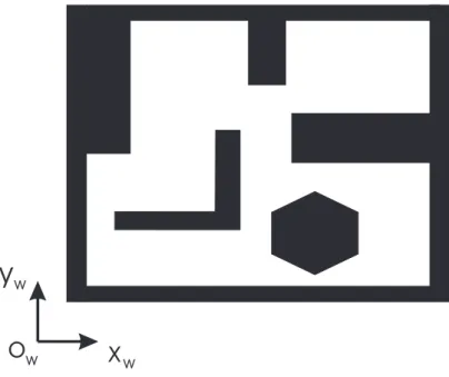
(3D), O = {O1, . . . , On}. Figure 2.1 shows a typical two-dimensional
workspace with a set of obstacles. This figure also shows the coordinate system, commonly called world reference frame{W}, which is used to localize obstacles and robots inside the workspace.
In the general case, there are two types of obstacles in a workspace:
2.1. WORKSPACE 10
x
wy
wo
wFigure 2.1: Typical mobile robot workspace.
static obstacles anddynamic obstacles. The former type corresponds to those obstacles that have fixed shapes, positions, and orientations over time. On the other hand, the latter type corresponds to those obstacles that have time-varying shapes, positions, and/or orientations. Normally, walls, trees, buildings, holes, and furniture are examples of static obstacles, while animals, other robots, and people are examples of dynamic obstacles.
2.2. CONFIGURATION SPACE 11
2.2
Configuration Space
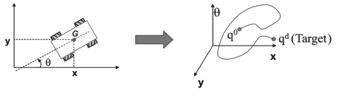
Given a robot R, a workspace W, and a world reference frame {W}, we define a configuration, q, as the vector of minimum dimension capable of completely characterize the robot’s placement in the workspace. For exam-ple, consider a mobile robot navigating in a planar surface, and a reference point Gwhich is fixed on the robot. The robot’s configuration q= [x, y, θ]T
is composed by the x and y coordinates of G and the robot’s orientation θ. Then, by definition, the configuration space,C, is the set of all possible con-figurations of the robot, while the robot’s trajectory is a continuous sequence of configurations in C. Figure 2.2 shows these concepts. The number of di-mensions of the configuration space corresponds to the number of degrees of freedom of the robot. Clearly, in Figure 2.2 we have three degrees of freedom. In the case of mobile robots navigating in three-dimensional workspaces, the configuration space has 6 dimensions, and the robots configurations may be represented byq= [x, y, z, α, β, θ]T. The first three dimensions correspond
to the cartesian coordinates of the reference pointG, and the other three are
Roll, Pitch, and Yaw angles. These angles define rotations around the axes
X, Y, and Z respectively of a body fixed frame.
Let {G} be a reference frame fixed at point G. Each configuration cor-responds to a homogeneous transformation matrix that converts points rep-resented in {G} to points represented in {W}. Such matrix can be written as:
WT
G =
WR
G WrO
01×m 1
, (2.1)
where WR
G is a rotation matrix that transforms the components of vectors
in {G} into components in {W}, Wr
O is the position vector of the origin of
2.2. CONFIGURATION SPACE 12
Figure 2.2: A robot is represented by a point in its configuration space. A trajectory is then a continuous sequence of configurations that starts at q0
(the initial robot’s configuration) and ends at qd (the desired final
configu-ration) [Pereira, 2003].
The set of all transformation matrices in m dimensions defines the so-called special Euclidean group, SE(m) [Murray et al., 1994]:
SE(m) =
T∈R(m+1)×(m+1)|T=
R r
01×m 1
, (2.2)
where R ∈ Rm×m, r ∈ Rm, RTR = RRT = I, and det(R) = 1. The
matrix I corresponds to the identity matrix and det(R) corresponds to the determinant of R.
Therefore, in the case of robots navigating in a planar surface we can say that q ∈ SE(2). This nomenclature just indicates that a configuration
q= [x, y, θ]T is equivalent to translations and rotations in 2D. Similarly, in
the case of the robot navigating in three-dimensional workspaces we can say that q∈SE(3).
The obstacles are represented in the robot’s configuration space as a set of forbidden configurations, Cobst. The computation of the robot’s
configu-ration space is usually performed by constructing the Cobst. This is done by
2.2. CONFIGURATION SPACE 13
Figure 2.3: Result of the growth of a rectangular obstacle by the size of a triangular robot with constant orientation [Pimenta, 2005].
not allowed to rotate. In this case, it is clear that the configuration space is two-dimensional. From Figure 2.3, we can conclude that it is possible to avoid collisions between the robot and the obstacle if we are able to limit the excursion of the point used to construct the Cobst in the configuration space.
When SE(2) or SE(3) spaces are considered, the complexity of the con-figuration spaces increases. The efficient computation of the robot’s config-uration space can be done by using Minkowski Sums [de Berg et al., 2000]. This technique was implemented in [Pimenta, 2005] and will be omitted here, since it is out of the scope of this thesis.
2.3. MOTION CONSTRAINTS 14
as the free configuration space, F [Latombe, 1991]:
F =C \ Cobst, (2.3)
Obviously, the objective of most approaches in robotics is to control the robot such that it never leaves F. An interesting approach that guarantees such condition is based on Navigation Functions which is presented later in this chapter.
2.3
Motion Constraints
It is very common that mechanical systems have their motion subjected to constraints. These constraints may arise from the structure of these mech-anisms, or from the way in which they are actuated and controlled. We will consider here only constraints that may be expressed as equalities and that are independent of time. Such constraints are called bilateral scleronomic
constraints [Luca and Oriolo, 1995].
Consider a n-dimensional configuration space, C. Constraints are called
holonomic if they may be put into the form
hi(q) = 0, (2.4)
where i = 1, . . . , k < n. For convenience, the functions hi : C → R are
assumed to be smooth and independent.
2.3. MOTION CONSTRAINTS 15
of n−k new coordinates that represent the actual degrees of freedom of the system.
Constraints that involve configurations, q, and velocities, ˙q, are named
Kinematic constraints. These constraints may be written as:
ai(q,q˙) = 0, (2.5)
where i= 1, . . . , k < n. If it is possible to put them into the form
aT
i (q)·q˙ = 0, (2.6)
then these constraints are referred to as Pfaffian constraints. Conveniently, the vector functions ai : C → Rn are assumed to be smooth and linearly
independent.
Holonomic constraints may always be put in the Pfaffian form by writing
aT
i =∂hi/∂q. However, the converse may not be true. Kinematic constraints
that are notintegrable, i.e., that cannot be put into the form (2.4) are called
nonholonomic constraints.
The effect of nonholonomic constraints is completely different from the effect of the holonomic ones. If a system is subjected only tok nonholonomic constraints then the number of dimensions of the configuration space is pre-served. On the other hand, the instantaneous system mobility is restricted to a (n−k)-dimensional subspace. In fact, such constraints limit the velocities that can be imposed to the system in a given instant of time.
2.3. MOTION CONSTRAINTS 16
2.3.1
Holonomic Mobile Robot
Holonomic mobile robots are those mobile robots which are subjected only to holonomic constraints. Therefore, the number of dimensions of the configuration space of these robots is reduced. On the other hand, there is no restriction on their instantaneous velocities in the reduced configuration space. This means that these robots can move in any desired direction in the reduced configuration space for all instants of time.
Consider a point robot in a 3D space that is only allowed to move in a planar surface. This surface defines a holonomic constraint for this robot. Suppose we place a cartesian reference frame with its origin located on the plane and with its z-axis perpendicular to the plane. Thus, it is clear that the plane may be completely described by the x and y coordinates and the holonomic constraint is given by z = 0. In the Pfaffian form:
[0,0,1]· ˙q= [0,0,1]·
˙
x
˙
y
˙
z
= 0. (2.7)
If the robot allows actuation directly in its velocities and (2.7) is the only constraint imposed, then this robot may be modelled by:
˙q=u(q, t), (2.8)
2.3. MOTION CONSTRAINTS 17
depend or not of time, t:
u(q, t) =
u1(q, t)
u2(q, t)
0
. (2.9)
If the robot provides acceleration inputs, then:
¨
q=u(q,˙q, t). (2.10)
In this case:
˙q = v,
˙v = u.
None of the models constrain the direction of movement on the plane.
2.3.2
Nonholonomic Robot
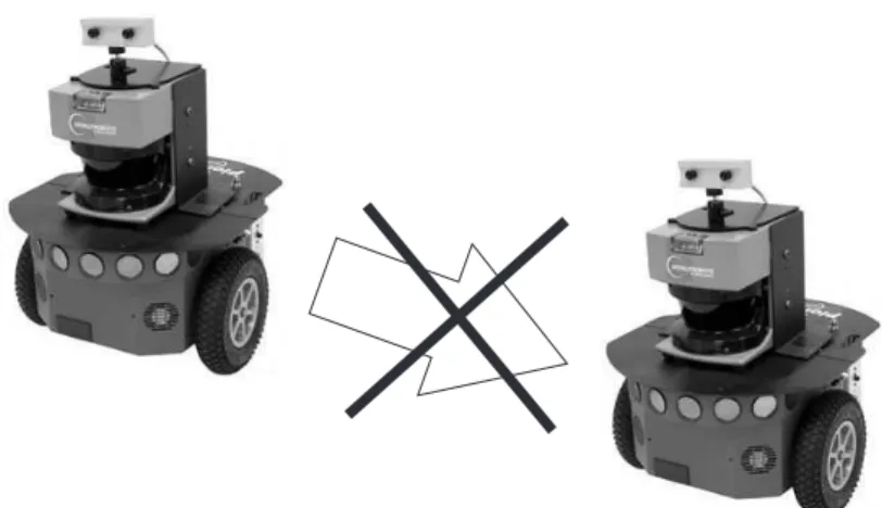
2.3. MOTION CONSTRAINTS 18
Figure 2.4: Nonholonomic constraint in differential drive robots.
motors.
If the robot is also subjected to the holonomic constraint mentioned be-fore, where the robot is confined to a planar surface, then we can assume
q = [x, y, θ]T and it is possible to characterize the nonholonomic constraint
of non-sideslipping using the following expression:
[sin(θ),−cos(θ),0]·
˙ x ˙ y ˙ θ
= 0, (2.11)
where θ is the robot orientation.
A kinematic model for this robot may be derived by considering the null space of the matrix AT = [sin(θ),−cos(θ),0]:
N = span
cos(θ) sin(θ)
2.4. LYAPUNOV STABILITY THEORY 19
The model is then given by
˙
q=
cos(θ) 0 sin(θ) 0
0 1
·
v
ω
, (2.13)
where v is the robot’s linear velocity and ω is the robot’s angular velocity. Since the relation between the speeds of the motors and v and ω is given by simple invertible algebraic expressions [Dudek and Jenkin, 2000], we can consider v and w as real control inputs. In fact, most commercial robots provide access only to these two variables.
2.4
Lyapunov Stability Theory
In this section we review some features of the Lyapunov Stability Theory
that will be used in the convergence proofs presented in Chapter 4. All definitions are given according to [Slotine and Li, 1991].
We will represent, in general, a nonlinear dynamic system by a set of n
nonlinear differential equations in the form:
˙
y=g(y, t), (2.14)
where g is a n ×1 nonlinear vector function, y is the n×1 state vector, and t is time. A solution of equation (2.14), y(t), corresponds to a curve in the state space. This curve is generally referred to as a state trajectory or a
system trajectory.
Nonlinear systems are traditionally classified as either autonomous or
2.4. LYAPUNOV STABILITY THEORY 20
Definition 2.1 (Autonomous and Non-autonomous systems) The
non-linear system in (2.14) is said to be autonomous ifgdoes not depend explicitly on time, i.e., if the system’s state equation can be written as
˙
y=g(y). (2.15)
Otherwise, the system is called non-autonomous.
In this work we will concentrate on autonomous systems. Therefore, the further definitions in this section assume systems of this type. The first important definition refers to a special class of system trajectory which cor-responds to only a single point. Such points are called equilibrium points.
Definition 2.2 (Equilibrium State or Equilibrium Point) A state y∗
is an equilibrium state (or equilibrium point) of the system if once y(t) =y∗,
it remains equal to y∗ for all future time. Mathematically, this means:
g(y∗) = 0. (2.16)
Equilibrium points can be classified as stable or unstable.
Definition 2.3 (Stable and Unstable Equilibrium Points) The
equilib-rium point y∗ is said to be stable if, for any δ > 0, there exists ǫ >0, such that if ky(0) − y∗k < ǫ, then ky(t) −y∗k < δ, ∀t ≥ 0. Otherwise, the
equilibrium point is unstable.
2.5. NAVIGATION FUNCTIONS 21
A generalization of the concept of equilibrium points is that of invariant sets.
Definition 2.4 A set G is an invariant set for a dynamic system if every system trajectory which starts from a point in G remains in G for all future time.
It is interesting to note that any equilibrium point is an invariant set. In fact, the whole domain of attraction of an equilibrium point is an invari-ant set. The following theorem allows for devising proofs of convergence of autonomous systems.
Theorem 2.1 (Local Invariant Set Theorem) Consider an autonomous
system of the form (2.15), with g continuous, and let V(y)be a scalar func-tion with continuous first partial derivatives. Assume that
• for some l >0, the region Gl defined by V(y)< l is bounded
• V˙(y)≤0 for all y in Gl
LetN be the set of all points withinGl whereV˙(y) = 0, andMbe the largest
invariant set in N. Then, every solution y(t) originating in Gl tends to M
as t → ∞.
Proof: Refer to [Slotine and Li, 1991].
In the above theorem, the word “largest” is understood as the union of all invariant sets within N.
2.5
Navigation Functions
2.5. NAVIGATION FUNCTIONS 22
Definition 2.5 (Robot motion planning problem) Let a single robotR
in the world W be represented by the configuration q ∈ C, and consider
F ⊆ C to be the free configuration space for R. Steer the robot from its initial configuration q0 ∈ F at time t = t
0 to the desired configuration qd ∈ F at
some time t=tf > t0, such that q∈ F ∀t ∈[t0, tf].
As pointed out in [Pereira, 2003], this problem consists of three basic subproblems: (i) computing the free configuration space, F, by considering the obstacles in W as described in Section 2.2; (ii) generating a trajectory
τ, which is a continuous sequence of configurations in F for R; and (iii) controlling the robot to followτ. In [Latombe, 1991], several solutions to the motion planning problem are presented.
One of the most popular techniques to plan trajectories and control robots in their configuration spaces is the Artificial Potential Field ap-proach [Khatib, 1986]. This apap-proach is based on the computation of a scalar potential function, φ(q), which is designed to have a minimum at the goal location and maxima at the boundaries of obstacles. The key idea is to use the descent gradient, −∇φ(q), to drive the robot to the goal. The descent gradient may be treated as a virtual force that simultaneously repels the robot from the obstacles and attracts the robot to the goal. This approach gives all possible trajectories independently of the initial configuration, since these trajectories are determined by the integral curves of the vector formed by−∇φ(q).
2.5. NAVIGATION FUNCTIONS 23
Figure 2.5: Local minimum caused by a U-shaped obstacle.
located, the robot is trapped inside the obstacle and never reaches the target. As proved in [Koditschek, 1987], it is impossible to find a smooth non-degenerate vector field1 on the configuration space of a point robot with m
obstacles admitting a globally asymptotically stable equilibrium state. In other words, it is impossible to find a global potential function with integral curves given by the descent gradient converging to the goal from every ini-tial configuration. However, it is possible to construct a potenini-tial function that is almost global, in the sense that the integral curves converge to the goal except from a set of measure zero2 initial configurations. It should be
clear that in the practical point of view such initial configurations are not problematic since they characterize saddle points. Therefore, they are unsta-ble equilibrium points and any perturbation compels the system to abandon them and converge to the goal.
Rimon and Koditschek [Rimon and Koditschek, 1988] devised special ar-tificial potential fields called Navigation Functions. Although saddle points are not prevented, these functions have a single minimum that coincides with
qd. A procedure to construct these navigation functions and also the
con-ditions of existence are given in [Rimon and Koditschek, 1992]. A potential
1
The vector field Jacobian matrix has full rank at the equilibrium points.
2
![Figure 1.1: Experiments with real robots. (a) Four robots caging a circular robot [Pereira, 2003]](https://thumb-eu.123doks.com/thumbv2/123dok_br/15791977.132587/39.892.191.705.189.390/figure-experiments-robots-robots-caging-circular-robot-pereira.webp)
![Figure 2.3: Result of the growth of a rectangular obstacle by the size of a triangular robot with constant orientation [Pimenta, 2005].](https://thumb-eu.123doks.com/thumbv2/123dok_br/15791977.132587/49.892.269.624.189.506/figure-result-rectangular-obstacle-triangular-constant-orientation-pimenta.webp)
![Figure 2.6: Path followed by an actual holonomic robot under the influence of a discretized harmonic field [Pimenta et al., 2006a].](https://thumb-eu.123doks.com/thumbv2/123dok_br/15791977.132587/64.892.307.586.189.582/figure-followed-actual-holonomic-influence-discretized-harmonic-pimenta.webp)