Mapping with MAV: Experimental Study on the Contribution of Absolute and Relative Aerial Position Control

Mapping with MAV: Experimental Study on the Contribution of Absolute and Relative

Aerial Position Control

Jan Skaloud a,_{, Martin Rehak} a_{, Derek Lichti} b

a

_{École Polytechnique Fédérale de Lausanne (EPFL), Switzerland - (jan.skaloud, martin.rehak)@epfl.ch}

b

_{The University of Calgary, Canada - ddlichti@ucalgary.ca}

KEY WORDS: Sensor orientation, MAV, Bundle adjustment, Relative aerial control

ABSTRACT:

This study highlights the benefit of precise aerial position control in the context of mapping using frame-based imagery taken by small UAVs. We execute several flights with a custom Micro Aerial Vehicle (MAV) octocopter over a small calibration field equipped with 90 signalized targets and 25 ground control points. The octocopter carries a consumer grade RGB camera, modified to insure precise GPS time stamping of each exposure, as well as a multi-frequency/constellation GNSS receiver. The GNSS antenna and camera are rigidly mounted together on a one-axis gimbal that allows control of the obliquity of the captured imagery. The presented experiments focus on including absolute and relative aerial control. We confirm practically that both approaches are very effective: the absolute control allows omission of ground control points while the relative requires only a minimum number of control points. Indeed, the latter method represents an attractive alternative in the context of MAVs for two reasons. First, the procedure is somewhat simplified (e.g. the lever-arm between the camera perspective and antenna phase centers does not need to be determined) and, second, its principle allows employing a single-frequency antenna and carrier-phase GNSS receiver. This reduces the cost of the system as well as the payload, which in turn increases the flying time.

1. INTRODUCTION

1.1 Motivation

The majority of today’s micro aerial vehicles (MAVs) employed for ortho-photo production, for example, use indirect sensor orientation. This method is very popular and effective whenever the surface texture allows for automated observation of (a large number of) tie-features. It is also relatively precise; however, its absolute accuracy is strongly related to the number of ground control points (GCPs) as well as their distribution within the block (Remondino et al., 2011; Vallet et al., 2011). Although the utilization of a large number of GCPs prevents model distortion, their establishment takes a substantial part of the mission budget. At the same time it is very well known that the precise observation of the camera perspective centers via global navigation satellite systems (GNSS) practically eliminates the need for GCPs in a block configuration of images, while improving its robustness and accuracy (Colomina, 1999). This so called AT-GNSS approach is often completed with a few GCPs to improve the redundancy and identify possible biases in GNSS positioning (Ackermann, 1992; Heipke et al., 2002). This technique called Integrated Sensor Orientation (ISO) or Assisted Aerial Triangulation (AAT) can be also extended for attitude aerial control and is likely the most common approach in the modern aerial triangulation with larger airborne platforms (Colomina, 2007).

As the employment of MAVs in aerial mapping is motivated by a rapidity and economy of data acquisition, the establishment of (a relatively high-number of) GCPs represents substantial

inconvenience and increases the operational budget especially in areas with difficult access. This motivates the presented investigations into removing the need for GCPs and/or reducing their number to a strict minimum.

1.2 Problem formulation

The traditional solutions for sensor orientation for MAVs are well known. In aero-triangulation (AT), a network of control and tie points is observed in a strip or block of images and each image’s orientation is estimated via bundle adjustment. In accuracy-demanding applications (e.g. cadastral) this requires establishment of ground control points across the whole area. On the other hand, direct sensor orientation eliminates the need for ground control points (and theoretically also for AT) as the absolute position and orientation of each image are directly observed with an integrated GNSS/IMU system. However, biases in the navigation data (e.g. due to incorrect carrier-phase ambiguity resolution) may occur and are sometimes difficult to detect. Their possible presence is habitually mitigated with additional modelling (e.g. shift and drift parameters) but requires GCPs, though fewer are required than for AT without aerial control (Blázquez and Colomina, 2012).

The inclusion of relative aerial control is a relatively new and rigorous approach to use INS/GNSS observations in airborne mapping (Blázquez, 2008). Its use was recently investigated on large aerial platforms with precise IMUs (Blázquez and Colomina, 2012). It is based on transferring the relative orientation of INS/GNSS system between two epochs to the relative orientation of a rigidly attached sensor between the The International Archives of the Photogrammetry, Remote Sensing and Spatial Information Sciences, Volume XL-3/W1, 2014

same two epochs. Although the concept is primary targeted for the combination of INS and GNSS observations, alternatively, only relative position models can be included in the bundle solution. In this approach, the bundle adjustment process cannot be completely eliminated, however, only a minimum number of GCPs is required. At the same time, the influence of the bore-sight misalignment can be neglected as well as that of the positioning bias. Since the observations are relative position vectors between images, the differencing operation removes the time-dependent biases provided. These could be considered as constant between two subsequent exposures. This offers the possibility to constrain the relative baselines within flight lines where the time period between successive exposures is short (typically dt < 5-10 s) while the satellite-receiver geometry does not vary significantly. In other words, if present, the position bias gets eliminated by the process of differencing without the need of additional modelling which may not correspond to reality (e.g. a drift is not linear within a flight-line). In the particular context of MAV, the aforementioned GNSS bias may occur not only due to the wrong ambiguities and/or unstable atmospheric conditions but also due to the local signal perturbations caused by the MAV electronics resulting in a lower signal-to-noise ratio (Mullenix, 2010). For these reasons we pay special attention to the method of relative aerial position control in this contribution.

1.3 Paper structure

The organization of the paper is as follows. After presenting a short review of photogrammetric models with absolute and relative aerial control, the paper highlights the challenges when integrating a carrier-phase, multi frequency GNSS receiver into a gimbal-suspended camera mount on board a MAV with vertical takeoff and landing (VTOL) capability. Then, a self-calibration of the camera’s interior orientation (IO) is performed. An independent flight with a small block of images is used to study the following test cases: indirect SO with 3 GCPs, integrated SO with 1 GCP using absolute-biased and absolute un-biased position aerial control from which corresponding relative position control is derived. Each case is evaluated with respect to 22 checkpoints distributed over the experimental area. The final part draws conclusions from the conducted research work and gives recommendations for future investigation.

2. OBSERVATION MODELS

2.1 Absolute position vectors

The observation equation that models the relation between the imaging sensor and the phase-centre of a GNSS antenna for which absolute position is derived takes the form:

l c c l c l l x l

S

N

A

R

X

v

x

     















_









1 , where (1)

the superscript

l

denotes a Cartesian mapping frame and the subscript

c

describes the camera frame,

l

x



1 is the GNSS-derived position (in our context derived from double-differencing) ,

l

x

v



are the GNSS observation residuals,

l

X



is the camera projection center,

l c

R

is the nine-elements rotation matrix from

c

to

l

frame,

c c

N

A

 



are the camera-antenna lever-arm and camera nodal distance, respectively and

l

S 

is the possible positioning bias in GNSS-derived position (e.g. wrong ambiguity, etc.). Time is a parameter for all

components in Eq. (1) with the exception ofAc 

andNc

 . If the time-tagging of camera exposure has a certain delay (dT) with

respect to GPS time, an additional factor l

v

dT shall be added

to Eq. (1), where

v

l is the velocity of the platform in the mapping frame. Such observation equations are included in the majority of commercially-available bundle adjustment software.

2.2 Relative position vectors

The observed base vector components between two camera centers 1 and 2,



_Xc_,Yc_,Zc



_{are parameterized in object} space as:                                              c c c c c c Z Y X c c c Z Y X Z Y X v v v Z Y X c c c 1 1 1 2 2 2 12 12 12

, where (2)

      c c

c _{Y Z}

X v v

v , , are the additive random errors. Assuming, that

the camera and GNSS antenna are rigidly mounted, the relative position vectors between successive perspective centres (base vectors) practically correspond to the base vector components in Eq. (2) and are easily derived from the two GNSS absolute positions Eq (1), i.e.:







_  _       _    

 c c

l c l c l l l x l l N A R R X X v x

x_{2 1 2 1 2 1} , where (3)

l l

x

x

  2

1

,

are the GNSS derived positions of two consecutive images, l l X X   2

1, are the camera projection centers of two consecutive

images. The parameterSl 

in Eq (1) can be considered as constant (at least over short period of time) is eliminated by differencing and therefore not present in Eq (3). Similarly to Eq (1), the observation Eq. (3) can be included in the bundle adjustment as weighted constraints, with weights derived rigorously from variance propagation. The remaining correlation between successive base vectors is, however, ignored.

2.3 Image observations

A pinhole camera model and the collinearity principle relate the observed image coordinates of a target

 

x

,

y

to the homologous object point (

l

-frame) coordinates



X,Y,Z



, the perspective centre (PC) coordinates



c c c



Z Y

X , , in

l

- frame, orientation The International Archives of the Photogrammetry, Remote Sensing and Spatial Information Sciences, Volume XL-3/W1, 2014

angles



,



,



encapsulated in the

r

_ijelements of the rotation

matrix l c

R

, the principal point co-ordinates (PP)



x_p,y_p



, the principal distance (PD) c and the distortion model corrections



x,y



and



vx,vy



are the additive random errors.



 

 





 

 



x

Z Z r Y Y r X X r Z Z r Y Y r X X r c x v x c c c c c c p

x 

             33 32 31 13 12

11 ₍₄₎



   





   



y

Z Z r Y Y r X X r Z Z r Y Y r X X r c y v

y _{c c c}

c c

c p

y 

             33 32 31 23 22

21 ₍₅₎

For the camera mounted on the MAV system a model comprising the first two radial lens distortion terms, k1 and k2, is sufficient to describe the imaging distortions. Hence in our case,







4



2 2 1r kr k x x

x  p  

 (6)







4



2 2 1r kr k y y

y  _p  

 (7)

,where



 

2



2

2

p

p y y

x x

r     .

3. CALIBRATION SETUP

3.1 Camera calibration

The aim of camera calibration is to determine the parameters of the interior orientation (IOs) that include the principal distance, the principal point offset and imaging distortion model coefficients, in particular those of the radial lens distortion model. Typically, self-calibration is performed in a laboratory and prior to mounting the camera in the MAV, by imaging a 3D field of targets in a strong geometric configuration. One of the reasons for this approach is that special network design measures (e.g. convergent imaging, roll diversity, completely filled image format) are required for a strong solution. These network design conditions are more easily achieved with the camera decoupled from the MAV platform. A preferable alternative is to calibrate the camera once installed on the platform in order to eliminate the need for dismounting it for regular calibrations. An airborne calibration still must incorporate the desired network geometry features. Some MAVs have the capability to incline the camera so as to acquire convergent imaging, but do so independently of the GNSS antenna, which disturbs the lever arm between the two devices and necessitates another calibration process. However, the presented MAV features a single mount that allows the camera and the antenna to be inclined together, thereby opening up the possibility for in-flight camera calibration with convergent imagery.

3.2 Self-calibration

As the details behind the self-calibration bundle adjustment procedure are well established they are not repeated here. See, for example (Fraser, 1997) for details. The network of images should include the aforementioned design features and its datum should be minimally constrained. The inner constraints (on object points) approach has been adopted here. Though the technological capabilities of the MAV system allow airborne calibration, the GNSS observations are not used as additional

observations in the self-calibrating bundle adjustment since they are not of sufficient quality to positively contribute to the adjustment.

3.3 Calibration field

A dedicated calibration field is approximately 20x25 meters large with height differences up to 2 meters. Ninety coded targets are distributed in a grid and the positions of 25 them are determined with sub-cm accuracy. The non-planar design of the target field decreases the correlation between the IO/EO parameters estimated through the process of self-calibration. The targets are digitally coded and their position in images is automatically recognized by utilizing an open-source libraries OpenCV and ARToolKit (Wagner and Schmalstieg, 2007).

4. DATA ACQUISITION

4.1 MAV

The drone used for this study is a custom made octocopter equipped with an open source autopilot (Rehak et al., 2013). The platform has a payload capacity up to 1.5 kg and flying endurance approximately 15 minutes. Various types of sensors can be attached rigidly on a sensor mount that pivots with respect to MAV body. Thanks to such construction, the positioning stability of camera-to-GNSS antenna is ensured as well as the ability to tilt the camera viewing direction along its lateral axis in order to capture images with various convergence angles. In addition, the mount is suspended to keep the sensor-head in level during the flight and to dampen the vibrations produced by the propulsion system.

4.2 Sensors

The chosen optical sensor onboard is the Sony NEX-5N camera. The quality and durability of this off-the-shelf camera has been proven during many UAV and UL (Ultralight airplanes) missions (Akhtman et al., 2013). For its size of 111x59x38 mm and weight of 210g (body only), the camera offers comparable image quality to considerably larger and heavier SLR cameras (Single-lens reflex). This makes it very suitable for UAV and MAV in particular. The chosen lens is a fixed 16 mm Sony lens, which has a reasonable optical quality for its size and weight and offers sufficient stability of the IO parameters throughput a mission.

We employ a geodetic-grade GPS/Glonass/Galileo multi-frequency OEM receiver from Javad with an appropriate antenna, RTK capability and 10Hz sampling frequency. A similar setup is used as a base station for carrier-phase differential processing.

4.3 Flown missions

Two flights were performed for the purpose of this study on different days and environmental conditions. The first mission was specifically for the camera calibration and resulted in a set of 92 images that were taken at two different flight levels (5 and 8 meters) and varying camera convergence angles. The second flight had a flying pattern similar to traditional photogrammetric flights with a nadir-looking camera. This set consists of 68 images taken from the altitude of 10 meters.

4.4 Processing strategy

The data recorded during the flight were pre-processed in a way similar to mature mapping systems. The image measurements were obtained from a custom script based on open-source libraries while the GNSS data was processed in a professional software package. Thanks to the precise time synchronization between the camera and the GNSS receiver, the exact acquisition time of each image is directly known and so absolute position vectors can be derived by interpolation from positioning solution at 10 Hz frequency and relative vectors obtained using Eq. (3). Within this study, the GNSS derived absolute and relative positions are used only in the second mission.

5. CASE STUDY

5.1 Camera self-calibration (flight I.)

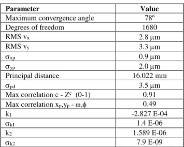
The most pertinent self-calibration results are summarized in Tab 1. The network is highly redundant with a large (by airborne standards) convergence angle. The measurement precision, as gauged by the root mean square (RMS) of the image point residuals, is a bit higher than might be expected at about 3 m (~1/2 of a pixel size). This can be attributed to degraded target measurement accuracy at oblique angles. Larger targets will be used in the future to improve the quality of image measurements. Nevertheless, a high precision calibration was achieved as the basic interior orientation parameter precision is on the order of a few m (after iterative variance component estimation). Importantly, the projection of the principal distance precision into object space at a typical flying height of 5 m is only 1.2 mm, which is an order of magnitude lower than the positional accuracy that can be achieved for a network oriented by GNSS. The principal point coordinates were successfully de-correlated from the angular orientation parameters while the principal distance still exhibits a maximum correlation coefficient with the height component of 0.91.

Table 1. Pertinent results from self-calibrating bundle adjustment

Parameter Value

Maximum convergence angle 78º

Degrees of freedom 1680

RMS vx 2.8 m

RMS vy 3.3 m

xp 0.9 m

yp 2.0 m

Principal distance 16.022 mm

pd 3.5 m

Max correlation c - Zc _{(0-1) 0.91}

Max correlation xp,yp - , 0.49

k1 -2.827 E-04

k1 1.4 E-06

k2 1.589 E-06

k2 7.9 E-09

5.2 Overview of test-cases (flight II.)

We created several network adjustment projects with various inputs to study the impact of different types of observations on the obtained mapping accuracy with respect to 22 checkpoints. All cases were run with fixed radial distortion parameters k1 and

k2 estimated during the preceding calibration project. The camera principal distance and the coordinates of the principal point were re-estimated to evoke a practical scenario. Indeed, the stability of both parameters cannot be guaranteed for different environmental conditions for such type of camera. For the projects with relative position observations, the last 6 (out of 68) absolute GNSS observations were used in order to eliminate the need of minimum ground control. Appropriate adaptations of the employed bundle adjustment software (Lichti and Chapman, 1997) were made to include observations of relative baseline vectors. The results of individual test cases are represented by overall RMS statistics and histograms of the residuals. Following summary describes these variants:

A. Aerial triangulation (AT) with three GCPs which are placed relatively close to each other, no aerial absolute or relative positioning control.

B. Assisted Aerial triangulation (AAT) with one GCP 1. Absolute aerial control (all 68 obs.) 2. Absolute aerial control (6 obs.) + Relative

aerial control (61 obs. with dt12 < 10s) C. Assisted Aerial triangulation (AAT) with one GCP

and degraded GNSS positioning quality 1. Absolute aerial control (all 68 obs.) 2. Absolute aerial control (6 obs.) + Relative

aerial control (61 obs. with dt12 < 10s) D. Assisted Aerial triangulation (AAT) with three GCPs

+ Relative aerial control (61 obs. with dt12 < 10s)

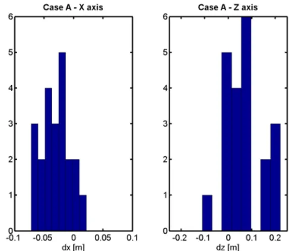
5.3 Case A: aerial triangulation with 3 close GCPs

The first case is focused on the indirect sensor orientation approach, which is the dominant method of sensor orientation when mapping with MAVs. Although the power of this concept is undisputable, it might be that due to the inaccessibility of the mapping area, only a limited number of GCPs can be established or their distribution does not extend over the whole field. To simulate this case the 3 selected GCPs were taken only from one-quarter of the mapped area. The outcome from the bundle adjustment for this case is presented in Tab. 2 and Fig. 1. The close spacing in the GCPs decreased the mapping accuracy in the rest of the field by a factor of 1.5-2 in comparison to the more optimal scenario and created a significant bias in the height component.

Table 2. Case A: Summary of indirect SO (AT + 3 close GCPs) on 22 checkpoints

Pos. residual

X [m] Y [m] Z [m]

MIN -0.072 -0.031 -0.110

MAX 0.021 0.073 0.221

MEAN -0.029 0.012 0.064

RMS 0.038 0.030 0.103

Figure 1. Case A: Histogram of residuals on the 22 check points

5.4 Case B: assisted aerial triangulation with one GCP and absolute (AAT/GNSS) and relative (AAT/R-GNSS) aerial control

The second case is focused on the contribution of the absolute and relative aerial control under optimal conditions. Although it is not essential in the absolute control, the inclusion of one GCP improves the redundancy and contributes to better re-determination of the focal length. This is a very expedient precaution since the camera principal distance should not be considered as a constant for the duration of one mission and has to be re-adjusted.

The quality of the GNSS positioning was checked independently with respect to the AT-derived camera positions using all 25 ground control points. Once accounting for the camera-antenna spatial offsets, the residuals between EO-positions are summarized in Tab. 3. The precision of direct positioning matches the expectations and corresponds to the accuracy of kinematic CP-DGPS.

Table 3. Summary of the quality of the GNSS data (determined with respect to indirect sensor orientation using all check points as ground control points)

Horizontal [m]

Vertical [m]

Mean estimated accuracy of GNSS positions

0.016 0.023 RMS of EO positions - estimated

(AT + 25 GCPs) vs. GNSS

0.020 0.039

Max GNSS residual 0.069 0.099

The statistic of residuals presented in Tab. 4 confirms that under ideal circumstances when there is indeed no bias present in the GNSS-derived absolute position, the differences between AAT/GNSS and AAT/R-GNSS seems negligible. Also the distribution of residuals, depicted in the Fig 2, stays within ± 7 cm boundary.

Table 4. Case B: Summary of ISO projects without bias

B1: ISO (AT + 1 GCP + 68 abs. GNSS)

residual X [m] Y [m] Z [m]

MIN -0.023 -0.040 -0.058

MAX 0.058 0.011 0.075

MEAN 0.011 -0.015 0.017

RMS 0.026 0.021 0.039

B2: ISO (AT + 1 GCP + 6 abs. GNSS + 61 rel. GNSS)

residual X [m] Y [m] Z [m]

MIN -0.018 -0.039 -0.079

MAX 0.059 0.014 0.070

MEAN 0.014 -0.015 0.006

RMS 0.027 0.021 0.039

Figure 2. Case B: Histogram of residuals on 22 checkpoints

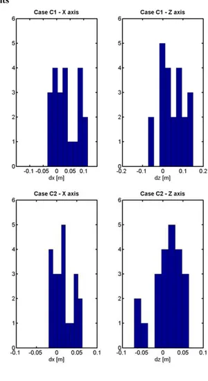
5.5 Case C: Assisted aerial triangulation with one GCP and absolute (AAT/GNSS) and relative (AAT/R-GNSS) aerial control for degraded GNSS positioning quality

Case C focuses on the most realistic scenario, when the quality of GNSS positioning is degraded and the ambiguities are not correctly resolved. In our case, we artificially reduced the number of available satellites to five for the 62 first exposures and maintained the last 6 exposures with the original number of observations. This resulted in systematic error in absolute positioning for the majority of the exposure stations. As shown in Tab. 5 and Fig. 3, the accuracy of AAT/GNSS worsens while that of AAT/R-GNSS is maintained.

This raises new options when employing GNSS-observations in a bundle adjustment. Practically, only few good positions are needed (minimum of 1) and those can be selected from epochs The International Archives of the Photogrammetry, Remote Sensing and Spatial Information Sciences, Volume XL-3/W1, 2014

where the number of tracked satellite is high and their geometry is strong. Alternatively, the minimum number of GCP (1) can be complemented by relative GNSS observations. These are less prone to carry an undetected bias (e.g. due to incorrect ambiguities) but enhance the strength of the whole network.

Table 5. Case C: Summary of integrated SO on projects with GNSS positioning bias

C1 : ISO (AT + 1 GCP + abs. GNSS + bias)

residual X [m] Y [m] Z [m]

MIN -0.034 -0.079 -0.072

MAX 0.115 0.011 0.150

MEAN 0.032 -0.037 0.047

RMS 0.055 0.046 0.073

C2: ISO (AT + 1 GCP + 6 abs. GNSS + 61 rel. GNSS + bias)

residual X [m] Y [m] Z [m]

MIN -0.020 -0.041 -0.071

MAX 0.063 0.014 0.065

MEAN 0.015 -0.016 0.010

RMS 0.029 0.022 0.038

5.6 Case D: Summary of integrated SO on project with GNSS positioning bias and relative GNSS observations

Case D repeats the case A to which relative aerial control of position is added. The 61 derived observations are taken from GNSS positions of degraded quality. In comparison to the case A, the residuals on check points (shown in Tab. 6) are 3-4 times lower in the horizontal components (< 1 cm!) and 3 times smaller in height.

Table 6. Case D: Summary of ISO (AT + 3 close GCPs + 61 relative GNSS + GNSS bias) on 22 checkpoints

Pos. residual

X [m] Y [m] Z [m]

MIN -0.006 -0.009 -0.087

MAX 0.012 0.020 0.058

MEAN 0.002 0.000 -0.007

RMS 0.005 0.007 0.036

Figure 3. Case C: Histogram of residuals on the 22 check points

6. CONCLUSION

This study highlighted the benefits of precise aerial position control in the context of a small UAV. Similarly to studies performed on larger platforms, the inclusion of precise observations of camera positions in MAV allowed to omit (or considerably reduce) the number of ground control points for the block of images. In cases when the quality of GNSS positioning is not high either due to the limited number of satellites in view, their sub-optimal geometry or low signal-to-noise ratio (SNR). The obtained results favour the approach of integrated sensor orientation with minimum GCPs and relative aerial control in position. In the case of MAV, the relative positioning represents additional important advantages as it allows to use a single-frequency carrier-phase GNSS receiver which is considerably smaller and cheaper.

7. REFERENCES

Ackermann, F., 1992. Operational rules and accuracy models for GPS aerial triangulation. Presented at the ISPRS, Washington, pp. 691–700.

Akhtman, Y., Rehak, M., Constantin, D., Tarasov, M., Lemmin, U., 2013. Remote sensing methodology for an ultralight plane. Presented at the 11th Swiss Geoscience Meeting, Lausanne, Switzerland.

Blázquez, M., 2008. A new approach to spatio-temporal calibration of multi-sensor system. Presented at the ISPRS Congress, International Archives of the Photogrammetry, Remote Sensing and Spatial Information Sciences, Beijing, China, pp. 481–486. Blázquez, M., Colomina, I., 2012. Relative INS/GNSS aerial

control in integrated sensor orientation: Models and performance. ISPRS J. Photogramm. Remote Sens. 67, 120–133.

Colomina, I., 1999. GPS, INS and Aerial Triangulation: what is the best way for the operational determination of photogrammetric image orientation? Presented at the ISPRS Conference Automatic Extraction of GIS Objects Digital Imagery, München.

Colomina, I., 2007. From Off-line to On-line Geocoding: the Evolution of Sensor Orientation. Photogrammetric Week’07, Wichmann, Germany.

Fraser, C.S., 1997. Digital camera self-calibration. ISPRS J. Photogramm. Remote Sens. 149–159.

Heipke, C., Jacobsen, K., Wegmann, H., 2002. Integrated sensor orientation: test report and workshop proceedings.

Lichti, D., Chapman, M.A., 1997. Constrained FEM self-calibration. Photogramm. Eng. Remote Sens. 63, 1111–1119.

Mullenix, D., 2010. Explanation of GPS/GNSS Drift. Ala. Precis. AG Agriculture, Natural Resources & Forestry.

Rehak, M., Mabillard, R., Skaloud, J., 2013. A micro-UAV with the capability of direct georeferencing. Presented at the UAVg, Rostock, Germany.

Remondino, F., Barazzetti, L., Nex, F., Scaioni, M., Sarazzi, D., 2011. UAV photogrammetry for mapping and 3D modeling-current status and future perspectives. Presented at the UAV-g 2011, Conference on Unmanned Aerial Vehicle in Geomatics, International Archives of the Photogrammetry, Remote Sensing and Spatial Information Sciences, Zurich, Switzerland. Vallet, J., Panissod, F., Strecha, C., Tracol, M., 2011.

Photogrammetric performance of an ultra light weight Swinglet “UAV”. Presented at the UAV-g 2011, Conference on Unmanned Aerial Vehicle in Geomatics, International Archives of the Photogrammetry, Remote Sensing and Spatial Information Sciences, Zurich, Switzerland.

Wagner, D., Schmalstieg, D., 2007. ARToolKitPlus for Pose Tracking on Mobile Devices. Presented at the 2th Computer Vision Winter Workshop, Sankt Lambrecht, Austria.