International Journal of Industrial Engineering Computations 6 (2015) 433–444
Contents lists available at GrowingScience
International Journal of Industrial Engineering Computations
homepage: www.GrowingScience.com/ijiec
Optimization of hole-making operations for injection mould using particle swarm
optimization algorithm
A. M. Dalavia*, P. J. Pawarb and T. P. Singha
aDepartment of Mechanical Engineering, Symbiosis Institute of Technology
, Symbiosis International University, Gram Lavale, Mulshi, Pune, India 412115
bDepartment of Production Engineering, K. K. Wagh Institute of Engineering Education and Research, Nashik, India
C H R O N I C L E A B S T R A C T
Article history: Received January 8 2015 Received in Revised Format May 10 2015
Accepted June 12 2015 Available online June 17 2015
Optimization of hole-making operations plays a crucial role in which tool travel and tool switch scheduling are the two major issues. Industrial applications such as moulds, dies, engine block etc. consist of large number of holes having different diameters, depths and surface finish. This results into to a large number of machining operations like drilling, reaming or tapping to achieve the final size of individual hole. Optimal sequence of operations and associated cutting speeds, which reduce the overall processing cost of these hole-making operations are essential to reach desirable products. In order to achieve this, an attempt is made by developing an effective methodology. An example of the injection mould is considered to demonstrate the proposed approach. The optimization of this example is carried out using recently developed particle swarm optimization (PSO) algorithm. The results obtained using PSO are compared with those obtained using tabu search method. It is observed that results obtained using PSO are slightly better than those obtained using tabu search method.
© 2015 Growing Science Ltd. All rights reserved
Keywords:
Hole-making operations Particle swarm optimization Injection mould
1. Introduction
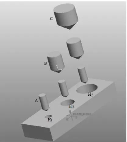
In machining process of many industrial parts such as dies and moulds, operations like drilling, reaming or tapping account for a large segment of process. Generally, a part, for e.g. a plastic injection mould may have many holes with different diameters, surface finish, and maybe various depths. If the diameter of hole is relatively large, a pilot hole may have to be drilled first using a tool of smaller diameter and then enlarge it to its final size with a larger tool, which could be followed by reaming or tapping whenever essential. For hole H3, as shown in Fig. 1, there could be four different combinations of tools:(A,B,C),
(A,C), (B,C), and (C). The selection of tool combinations for each hole directly influences on the optimum cutting speeds, required number of tools switches, and tool travel distance (Kolahan & Liang, 2000).
Fig. 1. Image showing various tool combinations required to drill a hole on workpiece
Tool switch and tool travel from one position to another takes more amount of machining time in machining processes. Usually 70% of the overall time in machining processes is spent on movements of tools and part (Merchant, 1985). To reduce the tool travel, the spindle is not moved until a hole is completely drilled using several tools in different diameters, which increases tool switching cost. On the other hand, to reduce tool switching cost, it may be used to drill all possible holes which, in turn, increases the tool travel cost. Luong and Spedding (1995) addressed the process planning and cost estimation of hole-making operations by developing a generic knowledge based procedure. Castelino et al. (2000) reported an algorithm for minimizing airtime for milling by optimally connecting various tool path segments. In their work, a problem was formulated as a generalized travelling salesmen problem and it was solved using a heuristic method. Kolahan and Liang (2000) introduced a tabu search approach to reduce the overall processing cost of hole-making operations. Alam et al. (2003) presented a practical application of computer-aided process planning (CAPP) system to reduce the overall processing time of injection moulds. Genetic algorithm (GA) was used for optimizing the selection of machine tools, cutting tools, and cutting conditions for different processes. Abu Qudeiri et al. (2007) used genetic algorithm to find the optimal sequence of operations which gives the shortest cutting tool travel path (CTTP).
Jiang et al.(2007) reported a stochastic convergence analysis of the parameters {ω, C1, C2} of standard
particle swarm optimization (PSO) algorithm. Shi et al. (2007) presented a novel PSO based algorithm for solving the travelling salesman problem (TSP). They compared their proposed algorithm with existing algorithms and found that PSO could be used for solving large size problems. Zhang et al. (2008) presented an improved PSO algorithm (IPSO) based on the “all different” constraint to solve the flow shop scheduling problem with the aim of minimizing make span. Guo et al. (2009) developed a problem on integration of process planning, scheduling of manufacturing field using PSO algorithm. Shao et al.
order exchange. Chandramouli et al. (2012) reported sheep flock heredity algorithm (SFHA) and artificial immune system (AIS) for reducing time of the scheduling of machines, an automated guided vehicle (AGV) and two robots in a flexible manufacturing system. Bhongade and Khodke (2012) proposed two heuristics for solving assembly flow shop scheduling problem. Shahsavari Pour et al. (2013) presented genetic algorithm for solving the flow shop scheduling problem.
Ghaiebi and Solimanpur (2007) applied ant colony optimization (ACO) algorithm for optimizing the sequence of hole-making operations of industrial part. Hsieh et al. (2011) used immune based evolutionary approach to find the optimal sequence of hole-making operations. Tamjidy et al. (2014) presented an evolutionary algorithm to reduce the tool travel and tool switching time during hole-making operations based on geographic distribution of biological organism.
It is revealed from the literature that non-traditional methods such as tabu search (TS), genetic algorithm, ant colony algorithm, immune algorithm (IA) etc. were used to solve the problem of optimization of hole-making operations. However, pure tabu search that uses only one solution can easily neglect some promising areas of the search space, and may also not find optimal or exact solution. Most commonly used advanced optimization techniques are the implementation for genetic algorithm in manufacturing optimization. Genetic algorithm (GA) gives near optimal solution for complex problems (Rao, 2011) and it requires more parameters (Elbeltagi et al., 2005). In ACO algorithm, convergence is slow due to pheromone evaporation and it tends to use more CPU time (Elbeltagi et al., 2005). Immune based evolutionary approach requires more parameters. Hence it is necessary to use non-traditional optimization algorithm, which gives correct solution for complex problems (Rao, 2011). From literature it is found that recently developed optimization algorithm known as PSO could be used due to its simplicity, easy implementation and high convergence rate (Coello et al., 2011). In this work an attempt has been made by using PSO to reduce overall processing cost of hole-making operations through determination optimal sequence for hole-making operations.
2. Formulation of an optimization model
In order to reduce the overall processing cost of hole-making operation, the following optimization model is formulated based on the analysis given by Kolahan and Liang (2000) considering the following components of overall processing cost:
2.1. Tool travel cost
Tool travel cost is the cost of moving the tool from its previous location to the current drilling location.
2.2. Tool switch cost
It occurs whenever a various tool is used for the next operation. If the required tool type is not available on the spindle for machining operation, then the required tool must be loaded on the spindle prior to performing a machining operation.
2.3. Tool and machining costs
Tool cost includes the new tool cost and the cost of machine down time required to replace the tool. Machining cost comprises the operating cost and the machine overhead cost. The combined tooling and machining costs when tool type m is used on hole j can be expressed as Eq. (1):
,
mj m mj mj
mj
Z
Yt
T
t
Y
=
×
+
where,
m, tool type index in ascending order according to the tool diameters, m=1,...,M
j,k,l, hole index, j=1,...,J k=1,...,J l=1,...,J
mj, index for the last tool to be used on hole j
Ymj, combined tool and machining costs when tool type m is used on hole j. tmj, machining time required by tool m for hole j
Tmj life of tool type m associated with cutting operation on hole j Zm, cost of tool type m
Y, machining cost per unit time
Machining time, tmj, is determined by Eq. (2):
,
1000 mj m
j m mj
f U
L d
t =
π
(2)where,
dm, diameter of tool m
Lj, depth of hole j, including the clearance
Umj, cutting speed of tool m associated with an operation on hole j fm, recommended feed rate for tool type m
In drilling operations depth of cut is fixed. In normal practice feed is kept as a constant rate of cutting speed. Hence the optimum cutting speed, Umj, for the constant feed rate can be obtained by solving the
following differential Eq. (3):
0
=
mj mj
dU
dY (3)
The cutting speed obtained from Eq. (3) reduces the sum of tool and machining costs for a single operation. Considering all aspects mentioned above the final optimization model can be expressed as given by Eqs. (4-6).
' '' ''
' '' j
'
'
m M 1 1 1 '
min ( ) min
2
j
J J J
lj jk mm j
m mm j
mm m ljk mm j
l j k
m M m M mm j
p p t
G s x a bq Z t Y
T
∈ ∈ ∈ = = =
+
= + + +
∑ ∑ ∑ ∑∑∑
(4)subject to
j
xmmmljk
J
k J
l M m
∀ =
∑
∑
∑
∑
= = ∈ ∈
1 '' ' ''
j 1 1
M m
(5)
1 '' ' ''
' + ≤
kjl m mm ljk m mm x
x {l, j,k,m,m',m''}l≠ j,k ≠ j,m∈Mj,m'∈Mj,m''∈Mj (6)
where,
s is the sequence index, denoting a specific permutation of operations, G(s) represents the overall cost associated with operations in sequence s, a denotes thecost per unit non-productive travelling distance,
b is associated with thecost per unit tool switch time, Mj, is a set of tools that can be used to drill hole j
to its final size, pjk, is non-productive travelling distance between hole j and hole k, qmm''j, represents tool
integer variable, i.e. xmm'm''ljk=1 if tool m replaces tool m" to drill hole j which is located in the path
between holes l and k and has been drilled by tool m'; 0, otherwise. The 0-1 decision variable, xmm'm''ljk
simultaneously determines the sequence of holes to be processed as well as the indices m, m', and m" are used to achieve the correct sequence of tools for machining of each hole. Constraint set (5) ensures that each hole is drilled to its final size. Constraint set (6) states that backward movement of spindle is not allowed unless a tool switch is needed. To solve this model large amount of computational time is required as relatively large number of 0-1 decision variables are involved. To overcome this problem, efficient solution procedure using PSO algorithm is proposed.
3. Particle Swarm Optimization (PSO) algorithm
Particle swarm optimization is an evolutionary computation technique developed by Kennedy and Eberhart (1995). The particle swarm thought was originated as a simulation of a simplified social system. This technique starts with initialization of population of random solutions called “particles”. This algorithm consists of two “best” values. First one is the “pbest” best fitness values of individual particles
achieved so far. Second is the “gbest” which is the one with the best values among all the particles.
Velocity and position of individual particles are obtained and updated using Eqs. (7-8) (Kennedy & Eberhart, 1995). Each particle updates its velocity and position through the problem space by comparing its current position and velocity with the optimal solution. In PSO, velocity of particles is changed at every generation towards the “pbest” and “gbest”.
) (
)
( 2 2
1 1
1 i besti i besti i i w V C r p X C r g X
V+ = × + × × − + × × − (7)
1
1 +
+ = i + i i X V
X (8)
where,
1
+ i
V = New velocity of each particle,
w = Inertia weight,
i
V =Previous velocity of particle,
1
r&r2=random numbers between 0 to 1,
1
C &C2= acceleration constants or Cognitive and social constants,
i
X = Previous position of particle.
The acceleration constants ‘Cl’ and ‘C2’ in Eq. (7) represent the weighting of the stochastic acceleration
terms that pull each particle towards ‘pbest’ and ‘gbest’ positions. Thus, tuning of these constants varies the
amount of tension in the system. Low values of the constants allow particles to pass through far from target regions before being tugged back, while high values result in rapid movement toward, or pass through target regions (Elbeltagi et al. 2005; Dong et al. 2005). The inertia weight ‘w’ plays a crucial role in the PSO convergence behavior since it is used to manage the exploration abilities of the swarm. The effect of w, C1 and C2 on convergence for standard numerical benchmark functions was provided by
Bergh and Engelbrecht (2006). The optimum selection of operating parameters of the algorithm like acceleration constants ‘C1’ and ‘C2’ as well as inertia weight ‘w’ is essential for the convergence of the
algorithm. To ensure the convergence of the PSO algorithm, the condition specified by the f Eq. (9) must be satisfied (Bergh & Engelbrecht, 2006):
max (|λ1|, |λ2|) <1 (9)
2 1 1 2 1
γ φ φ
λ = +w− − + , (10)
1 2
2
1
, 2
w φ φ γ
λ = + − − − (11)
where γ =
(
1+w−φ1−φ2)
2 −4w , φ1 = C1×r1 and φ2 = C2×r2.As the feasible range for w is 0-1 and for C1 and C2 is 0-2, the selected values of w, C1 and C2 should be
arranged such that the Eq. (9) is satisfied for all possible values of random numbers r1 and r2 in the range
0-1. The controlling parameters of PSO algorithm are selected based on the above mentioned criteria for the application example discussed in the next section.
4. Application Example
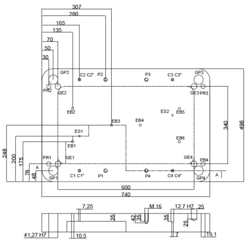
The particle swarm optimization algorithm is implemented to determine the optimal sequence of operations and corresponding cutting speeds of the upper holder of plastic injection mould as shown in Fig. 2 (Kolahan & Liang, 2000). The input data required for determining the optimal sequence of operations and corresponding cutting speeds of this mould using PSO are considered from (Kolahan & Liang, 2000).This mould consists of total 32 holes namely GP1, GP2, GP3, GP4, GE1-GE4, PR1-PR4, C1-C4, C1''-C4'', P1-P4, EB1-EB6, ES1-ES2. Fig. 2 also shows data related to the distances between the holes, type of operations required, and the depth of each hole.
Fig. 2. Upper holder of the plastic injection mould
Table 1
Data of tool diameter, cost, and specified feed rate considered for an application example.
Tool type m
Drill Reamer Tap
1 2 3 4 5 6 7 8 9 10 11 12
fm (mm/rev) 0.12 0.1 0.12 0.15 0.2 0.2 0.18 0.15 0.5 0.8 0.8 1.5 dm (mm) 7 7.25 10.5 12.5 13 19 25 41 12.7 19.1 41.2 16
Zm($) 10 12 15 15 14 20 26 50 55 70 85 45
5 7 . 0 4 . 0 ) 8 ( m mj m mj f U d T ×
= , for drilling a new hole
(12) 5 7 . 0 2 . 0 4 . 0 ) 4 . 18 ( m mj mj m mj f e U d T × ×
= , for enlarging a hole by drilling (13)
5 . 2 65 . 0 2 . 0 3 . 0 ) 1 . 12 ( m mj mj m mj f e U d T × ×
= , for enlarging a hole by reaming or tapping
(14)
where, emj, is depth of cut when tool type m performing a cutting operation on hole j. Optimum cutting
speeds expressed in Eqs.(15-17) can be achieved by solving differential Eq.(3) with Eqs. (12-14) (Kolahan & Liang, 2000):
5 5 . 3 2 6 m m m mj f Z Yd
U = × , for drilling a new hole
(15) 5 5 . 2 2 9 . 13 m mj m m mj f e Z Yd
U = × , for enlarging a hole by drilling
(16) 5 . 2 65 . 1 5 . 0 75 . 0 3 . 10 m mj m m mj f e Z Yd
U = × , for enlarging a hole by reaming or tapping
(17)
Tooling and machining costs of individual operations are calculated using optimum cutting speeds obtained using Eqs. (15-17). For this application example, tool switch times required for machining of hole-making operations are given in Table 2.
Table 2
Tool switch times (min)
Next in line Tool 1 2 3 4 5 Previous Tool 6 7 8 9 10 11 12
1 0 0.6 0.2 0.4 0.4 0.9 0.6 1 0.8 1.4 0.4 1
2 0.6 0 0.8 1.2 0.4 0.8 1.2 0.5 0.6 0.6 1.2 1.4
3 0.2 0.8 0 0.6 1.4 1.2 1.4 1 0.4 1 1.9 1.2
4 0.4 1.2 0.6 0 0.4 0.7 1 1.6 0.8 1.4 0.4 0.6
5 0.4 0.4 1.3 0.5 0 0.8 0.6 1 0.8 1.8 1.6 1.5
6 0.5 0.5 1.2 0.2 0.8 0 0.2 1.5 1.2 1.3 0.4 1.9
7 0.6 1.2 1.4 1 0.6 0.4 0 1 0.8 0.8 1.2 0.6
8 1 0.6 0.6 0.4 0.4 0.7 0.6 0 0.8 1.5 0.4 0.5
9 0.2 0.9 1.1 0.6 1.5 1.2 1.4 1 0 1.2 2 1.2
10 0.4 1.2 0.7 1.5 0.5 0.3 1 0.4 0.7 0 0.4 0.6
11 0.4 1.2 2 0.4 1.2 0.8 0.6 1.2 0.8 1 0 0.2
Table 3
Tool-hole combinations considered in the application example.
J GP1-GP4 GE1-GE4 PR1-PR4 C1-C4 C1''-C4'' P1-P4 EB1-EB6 ES1-ES2
mj 6-8-11 6-7 6-10 4-9 1 5-12 3 2
Table 3 corresponds to different combinations of tools necessary for machining of an individual hole to its final size as shown in Fig. 2. For example, holes GP1, GP2, GP3, GP4 require tool number 6 as initial tool, tool number 7 as intermediate tool and tool number 11 and a reamer to achieve the final size hole. Similarly, other holes involve a tool or different combinations of tools to achieve the final size hole. As given in Table 3, 56 machining operations are required for the example shown in Fig. 2. Process parameter assumed for this application example are, Y=$1/min, a=$0.0008/mm and b=$1/min.
5. Results and Discussion
For computational experiments, a Windows 8 PC with Intel core i3 CPU @ 1.90 GHz and Code blocks C compiler were used. In order to compare the results of PSO with those obtained using tabu search method developed by Kolahan and Liang (2000), for the application example considered in section 4, the following two cases are considered:
Case 1: Considering tool switch times given in Table 2,
Case 2: Considering tool switch times 50% of those given in Table 2,
Case 1: Following algorithm specific parameters for particle swarm optimization are obtained through various computational experiments.
C1=1.5, C2=2.0, w=0.5,
Number of iterations =500, Number of particles=100.
For the above parameter setting, the results of optimization for case 1 using PSO are given in Table 4.
Table 4
Results of optimal sequence of operation and associated cutting speeds for Case 1 using PSO
mj 6-GE2 6-GP2 6-PR2 6-PR1 6-GP1 6-GE1 6-GE3 6-GP3 6-PR3
Umj 33.016 33.016 33.016 33.016 33.016 33.016 33.016 33.016 33.016
mj 6-PR4 6-GE4 6-GP4 8-GP4 8-GP3 8-GP2 8-GP1 11-GP1 11-GP2
Umj 33.016 33.016 33.016 44.876 44.876 44.876 44.876 9.761 9.761
mj 11-GP3 10-PR3 10-PR4 10-PR1 10-PR2 7-GE3 7-GE2 7-GE1 1-C4''
Umj 9.761 9.622 9.622 9.622 9.622 49.675 49.675 49.675 36.372
mj 4-C4 9-C4 5-P4 5-P1 4-C1 4-C2 1-C2'' 1-C1'' 9-C1
Umj 36.177 11.13 30.464 30.464 36.177 36.177 36.372 36.372 11.13
mj 9-C2 5-P2 5-P3 12-P4 12-P3 12-P2 12-P1 7-GE4 11-GP4
Umj 11.13 30.464 30.464 3.642 3.642 3.642 3.642 49.675 9.761
mj 4-C3 1-C3'' 9-C3 3-EB5 3-EB1 3-EB3 3-EB2 3-EB4 3-EB6
Umj 36.177 36.372 11.13 39.444 39.444 39.444 39.444 39.444 39.444
mj 2-ES2 2-ES1
Table 4 corresponds to the optimal sequence of operations and associated cutting speeds of Case 1 that are obtained using PSO. This sequence results into overall processing cost of $66.78 including $45.2 machining and tool costs, $10.48 non-productive travelling cost, and $11.1 tool switch cost.
Fig. 3.a. Convergence of overall processing costs ($) of Case 1 using PSO
Case 2: The following algorithm specific parameters for particle swarm optimization are obtained through various computational experiments.
C1=1.65, C2=1.75, w=0.65,
Number of iterations =600, Number of particles=100.
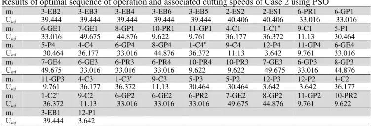
Table 5
Results of optimal sequence of operation and associated cutting speeds of Case 2 using PSO
mj 3-EB2 3-EB3 3-EB4 3-EB6 3-EB5 2-ES2 2-ES1 6-PR1 6-GP1
Umj 39.444 39.444 39.444 39.444 39.444 40.406 40.406 33.016 33.016
mj 6-GE1 7-GE1 8-GP1 10-PR1 11-GP1 4-C1 1-C1'' 9-C1 5-P1
Umj 33.016 49.675 44.876 9.622 9.761 36.177 36.372 11.13 30.464
mj 5-P4 4-C4 6-GP4 8-GP4 1-C4'' 9-C4 12-P4 11-GP4 6-GE4
Umj 30.464 36.177 33.016 44.876 36.372 11.13 3.642 9.761 33.016
mj 7-GE4 6-GE3 6-PR3 6-PR4 10-PR4 10-PR3 7-GE3 6-GP3 8-GP3
Umj 49.675 33.016 33.016 33.016 9.622 9.622 49.675 33.016 44.876
mj 11-GP3 4-C3 1-C3'' 9-C3 5-P3 5-P2 12-P3 12-P2 4-C2
Umj 9.761 36.177 36.372 11.13 30.464 30.464 3.642 3.642 36.177
mj 1-C2'' 9-C2 6-GP2 6-GE2 6-PR2 7-GE2 8-GP2 11-GP2 10-PR2
Umj 36.372 11.13 33.016 33.016 33.016 49.675 44.876 9.761 9.622
mj 3-EB1 12-P1
Umj 39.444 3.642
Table 5 corresponds to the optimal sequence of operations and associated cutting speeds of Case 2 that are obtained using PSO. This sequence results into an overall processing cost of $60.45 from which $45.2 is the tool cost and machining cost, $10.94 tool switch cost, and $4.31 tool travel cost.
0 10 20 30 40 50 60 70 80 90 100 1 1 7 3 3 4 9 6 5 8 1 9 7 1 1 3 1 2 9 1 4 5 1 6 1 1 7 7 1 9 3 2 0 9 2 2 5 2 4 1 2 5 7 2 7 3 2 8 9 3 0 5 3 2 1 3 3 7 3 5 3 3 6 9 3 8 5 4 0 1 4 1 7 4 3 3 4 4 9 4 6 5 4 8 1 4 9 7 5 1 3 5 2 9 T o tal P ro ce ss in g Cos t( $)
No. of Iterations
Fig. 3.b. Convergence of overall processing costs ($) of Case 2 using PSO
Table 6 shows comparison of results of application example obtained by using PSO algorithm and tabu search (Kolahan & Liang 2000).
Table 6
Comparison of results of optimization obtained by using PSO with those obtained by using tabu search Kolahan and Liang (2000) for Case 1 and Case 2
Case 1
Tooling and Machining Cost
Cmj ($)
Tool Travel Cost
($) Tool Switch Cost ($)
Overall Processing Cost ($)
Tabu Search (Kolahan and Liang2000) 45.2 11 8.6* 64.8
Tabu Search (Kolahan and Liang2000) 45.2 11 11.2** 67.4
PSO 45.2 10.48 11.1 66.78
Case 2
Tabu Search (Kolahan and Liang 2000) 45.2 4.9 10.1* 60.2
Tabu Search (Kolahan and Liang 2000) 45.2 4.9 13.15** 63.25
PSO 45.2 4.31 10.94 60.45
*Value wrongly calculated by Kolahan and Liang (2000).
**Corrected values obtained by substituting the optimum result obtained by Kolahan and Liang (2000) in Eq. (4)
The example of this application was originally solved by Kolahan and Liang (2000) using tabu-search approach in order to reduce the overall processing cost of hole-making operations. Sequence obtained using tabu-search for both cases is checked manually as given Eq. (4), it is observed that the actual tool switch cost for both cases is different than the results given by Kolahan and Liang (2000). Corrected results for both cases are given in Table 6. PSO results are compared with these corrected results given in Table 6.
6. Conclusion
Optimization of hole-making operations involves large number of hole-making operations sequences due to the location of hole and tool sequence constraint. To achieve this, proper determination operations sequence and associated cutting speeds which reduces the overall processing cost of hole-making operations are essential. In this paper, a methodology has been proposed to reduce the overall processing cost of hole-making operations of an application example using PSO algorithm. The obtained results
0 10 20 30 40 50 60 70 80 1 2 6 5 1 7 6 1 0 1 1 2 6 1 5 1 1 7 6 2 0 1 2 2 6 2 5 1 2 7 6 3 0 1 3 2 6 3 5 1 3 7 6 4 0 1 4 2 6 4 5 1 4 7 6 5 0 1 5 2 6 5 5 1 5 7 6 T o ta l P ro ce ss ing C o st ( $ )
No. of iterations
have been compared with those obtained using tabu-search approach reported by Kolahan and Liang (2000). It is observed that the results of optimization obtained by PSO algorithm were slightly better than tabu-search approach (Kolahan & Liang, 2000) since for both cases showing an improvement about 1.0% for Case 1 and 4.6 % for Case 2. However for the both cases, the sequence of operation to be performed shows significant changes with respect to results obtained using tabu-search approach (Kolahan & Liang 2000).This clearly shows that PSO algorithm has potential to solve this problem. Also it is observed that PSO algorithm requires only 600 generations to converge to optimal solution. The improvement obtained by using PSO algorithm is thus significant and clearly indicates the potential of this method to solve real life problems related to hole-making for various industrial applications.
Acknowledgment
The authors are thankful to Mr. Pankaj Paliwal, Assistant Professor, Mathematics department, Symbiosis Institute of Technology, Pune, for extending help while preparing C-language code.
References
Alam, M. R., Lee, K. S., Rahman, M., & Zhang, Y. F. (2003). Process planning optimization for the manufacture of injection moulds using a genetic algorithm. International journal of computer
integrated manufacturing, 16(3), 181-191.
Van Den Bergh, F. (2006). An analysis of particle swarm optimizers (Doctoral dissertation, University
of Pretoria).
Van den Bergh, F., & Engelbrecht, A. P. (2006). A study of particle swarm optimization particle
trajectories. Information sciences, 176(8), 937-971.
Bhongade A. S., & Khodke P.M. (2012) .Heuristics for production scheduling problem with machining and assembly operations. International Journal of Industrial Engineering Computations, 3, 185–198. Carlos A.Coello Coello, Gary B.Lamont & David A. Van Veldhuizen (2007). Evolutionary Algorithms
for Solving Multi-Objective Problems. Springer, 2nd ed., 584-593.
Castelino, K., D’Souza, R., & Wright, P.K. (2002). Tool path optimization for minimizing airtime during machining. Journal of Manufacturing Systems, 22(3),173-180.
Chandramouli A., ArunVikram M. S. and Ramaraj N. (2012). Evolutionary approaches for scheduling a flexible manufacturing system with automated guided vehicles and robots. International Journal of
Industrial Engineering Computations,3, 627–648.
Dong, Y., Tang, J., Xu, B., & Wang, D. (2005). An application of swarm optimization to nonlinear programming. Computers & Mathematics with Applications, 49(11), 1655-1668.
Eberhart R.C. & Shi Y. (2000). Comparing inertia weights and constriction factors in particle swarm optimization. In Proc. Congr. Evalutionary Computing, 84-89.
Elbeltagi, E., Hegazy, T., & Grierson, D. (2005). Comparison among five evolutionary-based optimization algorithms. Advanced engineering informatics, 19 (1), 43-53.
Ghaiebi, H., &Solimanpur, M. (2007). An ant algorithm for optimization of hole-making operations. Computers & Industrial Engineering, 52(2), 308-319.
Guo, Y.W., Li, W.D., Mileham, A.R., & Owen, G.W. (2009). Applications of particle swarm optimisation in integrated process planning and scheduling. Robotics and Computer-Integrated
Manufacturing, 25, 280–288.
Hsieh, Y. C., Lee, Y. C., & You, P. S. (2011). Using an effective immune based evolutionary approach for the optimal operation sequence of hole-making with multiple tools. Journal of Computational
Information Systems, 7(2), 411-418.
Jiang, M., Luo, Y.P., Yang. S.Y. (2007).Stochastic convergence analysis and parameter selection of the standard particle swarm optimization algorithm. Information Processing Letters,102, 8–16.
Abu Qudeiri, J., Yamamoto, H., &Ramli, R. (2007). Optimization of operation sequence in CNC machine tools using genetic algorithm. Journal of Advanced Mechanical Design, Systems, and
Kennedy, J. & Eberhart. R. (1995). Particle swarm optimization. Proceedings of IEEE International
Conference on Neural Networks, 4, 1942-1948.
Kolahan, F., & Liang, M. (2000). Optimization of hole-making operations: a tabu-search approach. International Journal of Machine Tools and Manufacture, 40 (12), 1735-1753.
Luong, L.H.S., &Spedding, T. (1995). An integrated system for process planning and cost estimation in hole-making. International Journal of Manufacturing Technology, 10, 411–415.
Merchant, R.L. (1985). World trends and prospects in manufacturing technology. International Journal
for Vehicle Design, 6, 121–138.
Rao, R. V. (2011). Modeling and optimization of modern machining processes. In Advanced Modeling
and Optimization of Manufacturing Processes (pp. 177-284). Springer London.
Shahsavari Pour N., R. Tavakkoli-Moghaddam & Asadi H. (2013).Optimizing a multi-objectives flow shop scheduling problem by a novel genetic algorithm. International Journal of Industrial
Engineering Computations,4, 345–354.
Shao, X., Li, X., Gao, L., & Zhang, C. (2009). Integration of process planning and scheduling—A modified genetic algorithm-based approach. Computers & Operations Research, 36, 2082 – 2096. Shi, X.H., Liang, Y.C., Lee, H.P., Lu, C., & Wang. Q.X. (2007). Particle swarm optimization-based
algorithms for TSP and generalized TSP. Information Processing Letters,103, 169–176.
Tamjidy, M., Paslar, S., Baharudin, B. H. T., Hong, T. S., & Ariffin, M. K. A. (2014). Biogeography based optimization (BBO) algorithm to minimise non-productive time during hole-making process. International Journal of Production Research, 1-15.
Zhang, C., Sun, J., Zhu, X., Yang, Q. (2008). An improved particle swarm optimization algorithm for flow shop scheduling problem. Information Processing Letters,108, 204–209.
Zhang, W-B., Zhu, G. (2011). Comparison and application of four versions of particle swarm optimization algorithms in the sequence optimization. Expert Systems with Applications, 38, 8858– 8864.