OBSERVATIONS ON THE PERFORMANCE OF X-RAY COMPUTED TOMOGRAPHY
FOR DIMENSIONAL METROLOGY
H.C. Corcorana,b,*, S.B. Brownb, S. Robsona, R.D. Spellerc, M.B. McCarthyb
a Department of Civil, Environmental and Geomatic Engineering, University College London, Gower Street, London, WC1E 6BT, UK - (h.corcoran.11, s.robson)@ucl.ac.uk
b National Physical Laboratory, Hampton Road, Teddington, TW11 0LW, UK - (stephen.brown, michael.mccarthy)@npl.co.uk
c Department of Medical Physics and Biomedical Engineering, University College London, Gower Street, London, WC1E 6BT, UK – [email protected]
Commission V, WG V/1
KEY WORDS: X-ray computed tomography (XCT), dimensional metrology, holeplate, orientation, beam hardening
ABSTRACT:
X-ray computed tomography (XCT) is a rising technology within many industries and sectors with a demand for dimensional metrology, defect, void analysis and reverse engineering. There are many variables that can affect the dimensional metrology of objects imaged using XCT, this paper focusses on the effects of beam hardening due to the orientation of the workpiece, in this case a holeplate, and the volume of material the X-rays travel through. Measurements discussed include unidirectional and bidirectional dimensions, radii of cylinders, fit point deviations of the fitted shapes and cylindricity. Results indicate that accuracy and precision of these dimensional measurements are affected in varying amounts, both by the amount of material the X-rays have travelled through and the orientation of the object.
1. INTRODUCTION
1.1 X-ray Computed Tomography
X-ray computed tomography (XCT) has its origins in the field of medicine and was invented in 1972 by Godfrey Hounsfield. However, due to its non-destructive nature it is increasingly being used in the manufacturing industry to measure dimensions and geometry along with being used for quality control and inspection. The rising nature of the technology has led to the need for increased accuracy and precision along with the characterisation of errors that occur during the imaging and reconstruction process. This will eventually lead to the results from XCT becoming traceable back to the SI unit, the metre. XCT is being used in areas such as: manufacturing, automotive, aerospace and geology, where the variety of materials being imaged includes: metals, plastic castings, additive manufacturing, electrical components, mummies and antiquities. The advantages of using XCT for dimensional metrology, are its ability to highlight defects and voids in a non-destructive manner of both traditional and additive manufactured parts along with reverse engineering and material composition analysis.
1.2 Basic Principles
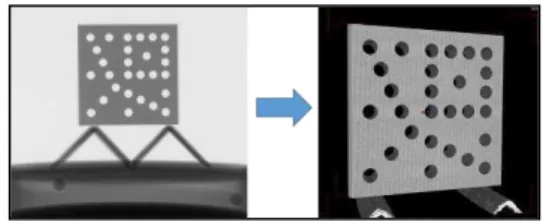
The basic principle of XCT is the attenuation of an X-ray as it travels through a material. This attenuation is a function of the path length and material that it is travelling through along with the X-ray energy. Attenuation is therefore related to the intensity of the X-ray that is measured on the detector after it has passed through the object. 2D images captured by the detector can be used in tomographic reconstruction to form a 3D volume using algorithms such as filtered back projection and the Radon transform, see Figure 1. The volume consists of voxels which ______________________
*Corresponding author
are like 3D pixels. They are representative of the attenuation of the object at that volume; the size of the voxel is related to the original pixel size of the detector and the magnification used.
Figure 1: 2D radiograph of the holeplate (on the left) and the reconstructed volume with surface determination A unit called ‘The Hounsfield unit’ is used to normalise the value for the calculated attenuation coefficient for each voxel and can be defined using equation 1.
��� ���=� ������������−�−��������� . (1)
where µmaterial = linear attenuation coefficient of material µwater = linear attenuation coefficient of water µair = linear attenuation coefficient of air
Traditionally 2D radiographs were used for taking measurements, to achieve this the rays that form the image must be reconstructed. This is achieved if the position of the focal spot in the X-ray source is known with respect to the plane of the image; this interior orientation is determined by calibration (American Society for Photogrammetry and Remote Sensing, 1989). For precise stereoscopic measurements targets must be positioned on and around the object, at least two images are then taken of the object from different orientations. This ties in with the principles used for XCT.
1.3 XCT Systems
Industrial XCT systems are comprised of many components, the main ones being an X-ray source, a manipulator to position and rotate the object being imaged and a detector. The basic layout can be seen in Figure 2.
The object is placed onto the manipulator and rotated, a series of images are taken of the different projections through the object. Changes in magnification can be achieved by moving the object towards or away from the source.
Figure 2: Typical cone beam XCT set up
Once the object has been reconstructed, a surface is defined by setting a threshold value, i.e. those voxels above a given value are defined as one material and those below another.
1.4 Variables
There are multiple variables that can affect dimensional measurement results, including those found with the system’s components (e.g. accuracy of positioning and stability of source)
and the workpiece’s shape and composition. These variables are
listed in the VDI/VDE (Association of German Engineers) document 2630 Part 1.2 (VDI/VDE-Richtlinien 2010) and many scientists are attempting to quantify them. This paper discusses the effects of the orientation of the object and the effect of beam hardening.
1.4.1Beam Hardening
As an X-ray beam passes through an object the lower energies are attenuated more than the higher energies, this leads to an increase in mean X-ray energy; this is known as beam hardening. This creates artefacts within the image known as cupping where the object is brighter at the edges and darker in the centre (Barrett & Keat 2004). It is only found in polychromatic X-ray beams that are composed of photons of multiple energies.
1.5 Reference Object
The use of XCT as a metrology tool in manufacturing has widespread use, it is therefore hard to develop a series of tests to mirror all objects and conditions where it is used. This study uses a simple holeplate (see Figure 3 for schematic) and some simple measurements that could be used in industry e.g. for holes in an engine block, to analyse errors found within the imaging and measurement process. Other more complex objects can be used but understanding the technology with simple objects is challenging enough.
The advantage of the simple holeplate is that it can be measured with a coordinate measuring machine (CMM) touch probe and measurements can be taken that relate to the ISO 10360 (ISO 2003) and for optical VDI/VDE 2617 document (VDI/VDE-Richtlinien 2014) which details testing of length measurement
errors. These tests are also similar to those carried out in measurements associated with photogrammetry.
The reference object, when used in different orientations, allows errors to be detected in the x, y and z axes.
2. METHOD
All experiments were carried out on a commercially available metrology XCT system with a maximum voltage of 225 kV and energy of 225 W. The manufacture states the MPE as (9 + L/50) µm where L is in mm.
2.1 Holeplate
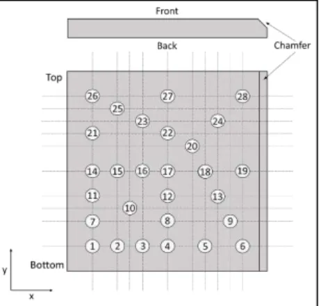
The National Physical Laboratory (NPL) holeplate was manufactured at NPL and is based on a design by Physikalisch-Technische Bundesanstalt (PTB) (Bartscher et al. 2014) to investigate the effects of beam hardening. It is made of aluminium and is (48 x 48 x 8) mm, the holes have a nominal radius of 2 mm. It was measured on a CMM, a Zeiss UPMC 550 (measurement accuracy (1.2 + L/400) µm) at NPL in order to compare the results obtained using the XCT.
The holeplate was imaged at three different orientations 0°, 45° and 90° to horizontal, horizontal being parallel to the x, z plane. It was supported in a carbon fibre frame and was placed on a plastic disk containing a calibrated ball bar of nominally 85.5 mm in length. Various voltages and currents were used for each set up in order to optimise the image quality. At the 90° orientation, the plate was placed on the rotary table with holes 1 to 6 uppermost. Images of the ball bar and holeplate were captured at the same time in order to check for any scaling errors of the XCT system. For these three different orientations it was also imaged at 5 differing magnifications, namely: 1.6, 2.0, 2.5, 3.0 and 3.5 creating voxel sizes of (125, 100, 80, 66.7 and 57.1) µm respectively.
Figure 3: NPL holeplate schematic indicating position of holes The images were reconstructed using the XCT manufacturer’s software. The resultant voxel data set was then imported into VGStudio Max, a commercial visualisation and analysis software for XCT data, developed by Volume Graphics GmbH. A surface was determined by initially defining the greyscale value for the air and the material interface, this surface was then used as a starting value for an algorithm that locally searches for the greatest rate of change in greyscale value between the two materials; this point is then defined as the new surface.
After the surface has been determined, cylinders are fitted to the holes using a Chebyshev fitting technique. All measurements are
taken from the reconstructed volume. The unidirectional cylinder centre to centre distances are recorded along with bidirectional distances, see Figure 4, cylinder radii and cylindricity. The deviation from the surface to the fitted cylinder are also logged for each fit point along with its x, y, and z coordinates. These coordinates were used to calculate the whole circle bearing around the cylinder of each fit point (see Figure 5).
Unidirectional Bidirectional
Threshold independent Edge independent Centre of cylinder is based on it being fitted with many points
Dependent on threshold setting
Influenced by material Based only on two points
Figure 4: Differences between unidirectional and bidirectional measurements
Figure 5: Orientation of holeplate during imaging and of whole circle bearing
3. RESULTS
3.1 Unidirectional and Bidirectional Lengths
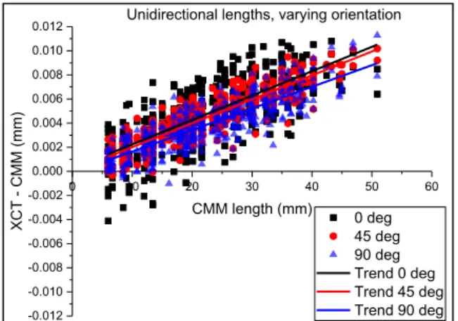
The results include unidirectional and bidirectional measurements. These are simple length measurements between various holes that can be used for comparisons of the holeplate at a fixed 1.6 times magnification but in the three chosen orientations. The graphs seen in Figure 6 and Figure 7 indicate that there appears to be a scaling error along the z axis. This suggests that the magnification used in the reconstruction process is incorrect. The error appears to have similar scaling influences on all three orientations.
Figure 6: Deviation between unidirectional lengths for holeplate at 1.6 times magnification in three orientations
Figure 7: Deviation between unidirectional lengths for holeplate at 1.6 times magnification in three orientations (using same
y axis scale as bidirectional graphs)
The scale factor can be determined by using the gradient of the trend in the data, the slope along with the standard deviation of the data can be seen in Figure 8.
Orientation Slope (mm) after scaling (mm)
0° 0.0002 0.0028 0.0020
45° 0.0002 0.0022 0.0010
90° 0.0002 0.0022 0.0012
Figure 8: Slope and standard deviation for deviation in unidirectional lengths taken at 1.6 times magnification The apparent scale error can be corrected using the gradient of the slope, the results can be seen in Figure 9.
Figure 9: Scaled deviation between unidirectional lengths for holeplate at 1.6 times magnification in three orientations The main difference between the measurements for the different orientations is that the spread is greater when the holeplate is at 0° than at 45° or 90°.
When comparing the bidirectional lengths, see Figure 10 the spread is greater than for the unidirectional dimensions. The standard deviations are an order of magnitude greater for the bidirectional measurements, see Figure 11. The scaling error is not so predominant, however, there is a positive systematic bias
0 10 20 30 40 50 60
-0.012 -0.010 -0.008 -0.006 -0.004 -0.002 0.000 0.002 0.004 0.006 0.008 0.010 0.012
0 deg 45 deg 90 deg Trend 0 deg Trend 45 deg Trend 90 deg
XCT -
CMM (
mm)
CMM length (mm)
Unidirectional lengths, varying orientation
0 10 20 30 40 50 60
-0.060 -0.040 -0.020 0.000 0.020 0.040 0.060
0 deg 45 deg 90 deg Trend 0 deg Trend 45 deg Trend 90 deg
XCT -
CMM (
mm)
CMM length (mm)
Unidirectional lengths, varying orientation
0 10 20 30 40 50 60
-0.012 -0.010 -0.008 -0.006 -0.004 -0.002 0.000 0.002 0.004 0.006 0.008 0.010 0.012
0 deg scaled 45 deg scaled 90 deg scaled
XCT -
CMM (
mm)
Scaled unidirectional lengths, varying orientations
CMM length (mm)
for 45° and 90°, whereas, when the holeplate is horizontal, there is a negative bias, i.e. the XCT data is measuring smaller in length than the CMM data.
Figure 10: Deviation between bidirectional lengths for holeplate at 1.6 times magnification in three orientations Orientation Slope (mm) after scaling
(mm)
0° 0.0002 0.0212 0.0210
45° 0.0001 0.0216 0.0216
90° 0.0000 0.0170 0.0169
Figure 11: Slope and standard deviation for deviation in bidirectional lengths taken at 1.6 times magnification Again the results were corrected for the scaling error, the results can be seen in Figure 12.
Figure 12: Scaled deviation between bidirectional lengths for holeplate at 1.6 times magnification in three orientations
3.2 Radii of Cylinders
The results comparing the deviation of the radii from the CMM data at 1.6 times magnification for the varying orientations can be seen in Figure 13 and Figure 14. They indicate that the most accurate results are achieved when the plate is angled at 45°, however the most precise results can be achieved when the plate is at 90°.
Figure 13: Deviation in cylinder radii at 1.6 times magnification using the cylinder fitted by Chebyshev fitting and
the CMM data Orientation Mean (mm) (mm)
0° -0.0105 0.0056
45° -0.0016 0.0024
90° 0.0148 0.0010
Figure 14: Mean and standard deviation for deviation in hole radii at varying orientations at 1.6 times magnification
3.3 Cylindricity
The cylindricity is a measure of straightness, roundness and taper and is measured by a feature being confined between two coaxial cylinders (ISO, 2012). The difference in the radii of the two cylinders should be as small as possible.
The authors are assuming that the holes are perfect cylinders. Results shown in Figure15, indicate that the perceived departure from cylindricity increases as the orientation of the holeplate increases. It also shows that at 45° the perceived cylindricity increases towards the centre of the holeplate and at 90° towards the lower holes. It should be noted that the holeplate was orientated such that holes 1 to 6 were viewed towards the top of the detector in the 45° and 90° orientation.
Figure 15: Cylindricity of cylinders compared to CMM data with varying orientation. (Width of circle proportional to
cylindricity)
10 20 30 40 50 60
-0.060 -0.040 -0.020 0.000 0.020 0.040 0.060
0 deg 45 deg 90 deg Trend 0 deg Trend 45 deg Trend 90 deg
XCT -
CMM (
mm)
CMM length (mm) Bidirectional lengths, varying orientation
10 20 30 40 50 60
-0.060 -0.040 -0.020 0.000 0.020 0.040 0.060
0 deg scaled 45 deg scaled 90 deg scaled
XCT -
CMM (
mm)
CMM length (mm)
Scaled bidirectional lengths, varying orientation
0 5 10 15 20 25 30
-0.020 -0.015 -0.010 -0.005 0.000 0.005 0.010 0.015 0.020
0 deg 45 deg 90 deg
XCT -
CMM (
mm)
Hole number
Radii of cylinders, varying orientation
3.4 Fit Point Deviations
To determine the shape of the cylinders the bearing, see Figure
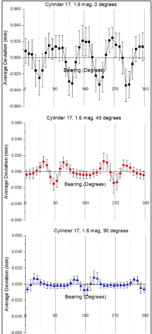
5, of the fit points was plotted against an average deviation taken every 10°, the results can be seen in Figure 16 and Figure 17 for cylinders 6 and 17. Again, both the spread and standard deviation decreases as the orientation of the holeplate increases (0°, 45° and 90°).
As well as a change in spread there are also peaks and troughs at differing angles around the cylinder. When the holeplate is lying horizontally (0°) the main trough for cylinder 6, with an average deviations of 32 µm, is at a bearing of 225°. At an orientation of 45°, there are two troughs with average deviations of up to 15 µm at a bearing of 90° and 270°, either side of these troughs are peaks of up to 12 µm. At 90° orientation the main two troughs, with average deviations of up to 10 µm, are at 180° and 0°/360°, there are also significant peaks of up to 10 µm either side of these two troughs.
Figure 16: Average deviation, taken every 10⁰, of fit point of cylinder 6 to surface. Error bars are equal to the standard
deviation.
For Figure 17, where cylinder 17 is in the centre of the holeplate, the results at 0° orientation are different from cylinder 6 at 0°. For Cylinder 17 at 0° there are four sets of peaks and troughs, unlike cylinder 6 at 0°where there are only two sets.
For orientations 45° and 90° the trends are very similar for cylinders 6 and 17, the main difference being that they are much more symmetrical for the cylinder 17 compared to cylinder 6.
Figure 17: Average deviation, taken every 10⁰, of fit point of cylinder 17 to surface. Error bars are equal to the standard
deviation.
4. DISCUSSION
The results indicate that this series of tests is useful to characterise both systematic and random errors occurring within the imaging and measurement process.
All of the results indicate that the noise is greatest when the plate is lying flat at 0° compared to 45° and 90°. Both the length measurements (unidirectional and bidirectional), radii and fit
point deviations show the greatest spread in data at the 0° orientation. The greatest error in cylindricity is also found at 0°, indicating that the greater the amount of material that the X-rays have to travel through, the greater the noise on the data. The spread in data for both unidirectional and bidirectional length shows similar values for 45° and 90°. The data becomes more precise as the orientation of the hole plate increases when studying the radii of the cylinders and the fit point deviations.
4.1 Systematic Errors
The various measurements highlight the systematic errors that are occurring during this measurement process.
4.1.1Unidirectional and Bidirectional Lengths
The scaling error that is apparent in unidirectional and bidirectional data is a systematic error that can be accounted for and corrected, see Figure 9 and Figure 12. This error appears to be caused by an error in the z axis and would become more problematic the larger the length being measured, i.e. the deviations between measured and true values would increase as the length increased.
After the scaling error has been corrected the results become more accurate for the unidirectional lengths, this, however, is not the case with the bidirectional lengths.
The larger spread of bidirectional results indicates that the threshold plays a crucial role when determining dimensional measurements. It also shows that larger errors are introduced when a single point, on the surface, is used for measurements. The use of unidirectional measurements that use the centres of fitted shapes reduces the influence of the threshold as the centre is independent of the size of the shape; assuming the shape’s centre is correct. There is an offset in the accuracy of the results, 0° shows a negative bias of approximately 20 µm and 90° shows a positive bias, also of 20 µm.
4.1.2Radii of Cylinders
Deviations for the radii appear to be systematic with regards to the orientation of the holeplate; the error is dependent on the orientation. The position of an imaged hole on the detector is independent of the radii measured, this is shown by cylinder 17, which despite being imaged on the same part of the detector, has three different radii which are dependent on the orientation of the holeplate. The small spread of the 90° results also indicate that the error is not caused by an error in the y axis, as, if this was the case, the radii would vary up or down the holeplate.
The offset in the radii depending on the orientation of the plate is a major question that needs to be answered. The error is crucial when imaging complex objects which may have features at varying orientations within it.
4.1.3Fit Point Deviations
The thickness of material appears to affect the fit of the cylinders, leading to a cyclic error in the deviations, this is particularly seen in cylinder 17 at 0° orientation. The troughs occur every time the corners of the holeplate are lined up with the source and detector, i.e. when the X-rays are travelling through the most amount of material. The peaks (when the surface is inside the fitted cylinder) occur when there is minimum material to travel through. It is interesting to note the variation in peaks for cylinder 17 at 0° orientation can be seen at 90° and 270°, at this time a reason for this is yet to be decided. Meganck et al. (2009) have
shown effects caused by beam hardening increase as the thickness of the material increases.
The relationship between the angles where the deviations are greatest and the orientation of the holeplate may be systematic, but at this time, with the information given, it cannot be proven so will be discussed further in 4.2.2.
4.2 Random Errors
Random errors cannot be corrected for, and may cause the results to be both inaccurate and imprecise.
4.2.1 Cylindricity
The increased deviation value in fit points leads to the increase in cylindricity as the orientation of the holeplate decreases (90°, 45° and 0°). If the major axis of the elliptical shape is increasing the cylindricity would have to increase to accommodate this. For all orientations the cylindricity offset is not constant for the different holes so could be classed as a random error.
4.2.2 Fit Point Deviations
Deviations at 90° and 270° when the holeplate is at 45° correspond to when the beam is travelling through the most material as the object rotates at this given orientation. This, however, is not the case when the object is at 90°, in this case the maximum deviations are clustered around 0°/360° and 180°. This may be as a result of not enough X-rays intersecting through the upper and lower surface of the hole, leading to the Tuy-Smith condition not being met as found by Hiller et al. (2010) leading to a loss of spatial resolution.
The fit point deviations for Figure 16 do not have the expected symmetry when the holeplate is at 0° orientation compared to when the holeplate is at 45° and 90°.
This lack of prediction in the deviations can therefore be counted as a random error because at this point there does not appear to be a constant error that could be accounted for.
4.3 Noise
Figure 18 highlights the change in profile shapes at the different orientations of the holeplate.
Figure 18: Profiles of greyscale through cylinder 6 going horizontally. Left to right 0⁰, 45⁰ and 90⁰. (Please note the
change in greyscale values on the y axis)
Figure 18, extracted from VGStudio Max, is indicative of the different levels of noise shown in the data sets and the relationship between the noise and orientation. The noise is far greater when the holeplate is at an orientation of 0° compared to 45° and 90°, this could lead to the threshold being set incorrectly.
5. CONCLUSIONS
As shown throughout, the series of graphs presented in this report show there is a correlation between the orientation of the holeplate and the noise of the data. Errors are both systematic and random. The systematic errors such as scaling can be corrected for, however, the random errors such as the variation in radii cannot be correct for, i.e. the deviation does not increase away from the correct value with orientation. Fundamentally the noise appears to be dependent on the amount of material the X-rays have had to travel through.
The random errors have to be investigated further in order to understand and characterise them into systematic errors in order to be able to work towards traceability of XCT dimensional measurements. International efforts are already under way to develop this understanding using many different reference objects. Use of a holeplate is just one reference artefact to be considered.
ACKNOWLEDGEMENTS
This research is based on a collaborative project funded by the EPSRC (Engineering and Physical Sciences Research Council) and the National Physical Laboratory through the VEIV (Virtual Environments Imaging and Visualisation) Engineering Doctorate Centre at University College London.
REFERENCES
American Society for Photogrammetry and Remote Sensing, 1989. Non-Topographic Photogrammetry 2nd ed. Karara H.M., ed., Virginia: American Society for Photogrammetry and Remote Sensing.
Barrett, J.F. & Keat, N., 2004. Artifacts in CT: recognition and avoidance. Radiographics : a review publication of the
Radiological Society of North America, Inc, 24(6),
pp.1679–91. Available at:
http://pubs.rsna.org/doi/full/10.1148/rg.246045065. Bartscher, M. et al., 2014. Current state of standardization in the
field of dimensional computed tomography. Measurement
Science and Technology, 25(6), p.064013. Available at:
http://stacks.iop.org/0957-0233/25/i=6/a=064013?key=crossref.eea8d55393859a71 4f2374d8b490133a.
Hiller, J. et al., 2010. Comparison of Probing Error in Dimensional Measurement by Means of 3D Computed Tomography with Circular and Helical Sampling. In 2nd
International Symposium on NDT in Aerospace.
Hamburg, pp. 1–7.
ISO, 2003. Geometrical Product Specifications (GPS) – Acceptance and reverification tests for coordinate
measuring machines (CMM) – Part 1: (ISO 10360-1:2000
+ Cor.1:2002).
ISO, 2012. Geometrical product specifications (GPS) —
Geometrical tolerancing — Tolerances of form,
orientation, location and run-out, (ISO 1101:2012)
Meganck, J.A. et al., 2009. Beam hardening artifacts in micro-computed tomography scanning can be reduced by X-ray beam filtration and the resulting images can be used to accurately measure BMD. Bone, 45(6), pp.1104–1116. Available at:
http://dx.doi.org/10.1016/j.bone.2009.07.078.
VDI/VDE-Richtlinien, 2014. VDI 2617-2.1 Accuracy of coordinate measuring machines parameters and their
reverification, Dusseldorf.
VDI/VDE-Richtlinien, 2010. VDI 2630-1.2 Computed
tomography in dimensional measurements, Dusseldorf.
Revised April 2016