Changes in climate, catchment vegetation and hydrogeology as the causes
of dramatic lake-level fluctuations in the Kurtna Lake District,
NE Estonia
Marko Vainu and Jaanus Terasmaa
Institute of Ecology, Tallinn University, Uus-Sadama 5, 10120 Tallinn, Estonia; [email protected], [email protected] Received 25 March 2013, accepted 2 October 2013
Abstract. Numerous lakes in the world serve as sensitive indicators of climate change. Water levels for lakes Ahnejärv and Martiska, two vulnerable oligotrophic closed-basin lakes on sandy plains in northeastern Estonia, fell more than 3 m in 1946– 1987 and rose up to 2 m by 2009. Earlier studies indicated that changes in rates of groundwater abstraction were primarily responsible for the changes, but scientifically sound explanations for water-level fluctuations were still lacking. Despite the inconsistent water-level dataset, we were able to assess the importance of changing climate, catchment vegetation and hydrogeology in water-level fluctuations in these lakes. Our results from water-balance simulations indicate that before the initiation of groundwater abstraction in 1972 a change in the vegetation composition on the catchments triggered the lake-level decrease. The water-level rise in 1990–2009 was caused, in addition to the reduction of groundwater abstraction rates, by increased precipitation and decreased evaporation. The results stress that climate, catchment vegetation and hydrogeology must all be considered while evaluating the causes of modern water-level changes in lakes.
Key words: lake-level fluctuations, groundwater abstraction, climate change, catchment, water balance.
INTRODUCTION
Lakes are important habitats for a variety of species and have a high recreational value for people. Abrupt changes in the water level of lakes affect both their ecological and recreational value, presumably in a negative direction. Therefore the mechanisms that affect the formation of the amount of water in a lake and the functioning principles of these mechanisms have to be understood in order to predict/prevent changes triggered by natural or anthropogenic causes.
In stable climatic and hydrogeological conditions the volume of a lake is considered to be in an equilibrium state (Street-Perrott & Harrison 1985). It means that lake volume may fluctuate annually because of seasonal changes in meteorological conditions, but the long-term average volume remains the same. Due to changes in catchment properties (vegetation, soil, topography) and climatic or hydrogeological conditions, the long-term average (equilibrium) volume of a lake may increase or decrease. The lake volume reaches a new equilibrium state when the triggering conditions stabilize again (Vassiljev 2007). To understand and explain the reasons behind these changes, the processes that affect the formation of the amount of water in a lake have to be known and decoded.
Climate change has been considered to be one of the main reasons for lake-level fluctuations (Adrian et al. 2009). The occurrence of a number of distinct climatic oscillations in Europe and their impact on lake levels has been widely studied in palaeolimnology (Digerfeldt 1986; Almquist-Jacobson 1995; Yu & Harrison 1995; Dearing 1997; Magny et al. 2001; Korhola et al. 2002; Punning et al. 2005; Kaakinen et al. 2010; Terasmaa 2011; Bjerring et al. 2013; Terasmaa et al. 2013). In neolimnological investigations the impact of future climate change on lake water budgets has also received considerable attention (George et al. 2007; Smith et al. 2008; Cardille et al. 2009; Taner et al. 2011). However, studies connecting recent lake-level changes to climatic shifts concentrate mostly on large lakes (Mercier et al. 2002; Anda & Varga 2010; Abbaspour et al. 2012; Lemoalle et al. 2012).
63
et al. 2008). Only a few studies suggest that the impact of vegetation change on runoff is insignificant (Peń a-Arancibia et al. 2012).
The impact of groundwater on lakes has long been considered insignificant, but has started to receive more and more interest. Winter et al. (1998) have called lake water and groundwater a single resource, pointing out that while studying the hydrology of a lake, one cannot neglect groundwater. Other researchers as well have stressed that, in order to ensure effective management of water resources and to explain changes in lake volumes, it is necessary to understand the basic principles of the interaction between groundwater and surface water (Hayashi & Rosenberry 2002; Sophocleous 2002; Gleeson et al. 2009).
In order to assess the effect of changes in climate, catchment vegetation or hydrogeology on lakes in the past or in the future, all the components of lake water balance have to be numerically determined. Lake water-balance studies use models that can be classified as deterministic or stochastic, conceptual or empirical, lumped or spatially distributed (Vassiljev 2007). The models (e.g. Hostetler & Bartlein 1990; Vassiljev et al. 1994, 1998; Cardille et al. 2004; Manley et al. 2008; Perrone et al. 2008; Reta 2011) vary in complexity and therefore in their applicability. Mainly because the existing models either required input data that were unavailable for the lakes studied by us (e.g. lake surface temperature, lake bed hydraulic conductivity) or did not cover all the necessary factors (e.g. filtration through the lake bed, catchment vegetation), a simple deterministic conceptual lumped spreadsheet-based tool for lake water-balance estimation had to be compiled for this study.
The aim of the current study is to assess the importance of changing climate, catchment vegetation and hydrogeology in water-level fluctuations in closed-basin lakes, which have scarce water-level data. Two closely situated lakes in NE Estonia, Lake Ahnejärv (hereafter L. Ahnejärv) and Lake Martiska (hereafter L. Martiska) were chosen as examples. Earlier investigations (Ilomets et al. 1987; Punning 1994; Punning et al. 2006, 2007) show that these lakes experienced a major water-level change during the previous century. In those papers the lake-level changes were qualitatively explained by the effect of groundwater abstraction that started near the lakes in the 1970s, but scientifically sound explanations for water-level fluctuations are still lacking. Although the wider aim of the study is to contribute to a general understanding of the causes of modern lake-level fluctuations, these specific lakes need special attention because they are a part of a Special Area of Protection created according to the European Union Habitats Directive (92/43/EEC). Severe water-level fluctuations endanger their preservation.
Three research objectives were delineated: (1) to evaluate the role of changes in catchment vegetation in lake-level fluctuations, (2) to assess the importance of changes in meteorological conditions in lake-level fluctuations and (3) to evaluate the effect of changes in hydrogeological conditions on the difference in lake-level rise at L. Martiska compared to L. Ahnejärv. An MS Excel-based water-balance tool was used to fulfil these objectives.
STUDY AREA
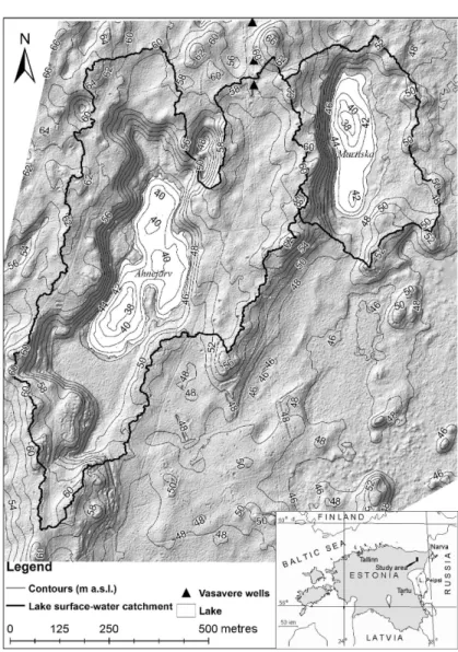
The study focused on two small lakes in the Kurtna Kame Field in NE Estonia, L. Ahnejärv and L. Martiska (Fig. 1, Table 1), which belong to the Natura 2000 network of Special Areas of Protection in the European Union. The Kurtna Kame Field (15 km2) is situated in a transitional zone between a sparsely inhabited territory with forests and mires and a heavily industrialized oil shale mining and processing region. The lakes are a part of the Kurtna Lake District that consists of 40 small lakes located in a 30 km2 area in and around the Kurtna Kame Field, which is featured by hillocks and small ridges, formed of bedded sand and gravel. The kame field has formed above the deep (up to 105 m) Vasavere valley that is filled with Quaternary deposits. Kames and the depressions between them are surrounded by limnoglacial and mire plains (Punning 1994). The lakes and the kame field belong to a landscape reserve. Both of the studied lakes have no surface water inlets or outlets (Fig. 1), but should have groundwater through-flow according to regional groundwater maps (Häelm 2010).
The surface-water catchments of both lakes are almost fully covered with a ca 60-year-old pine forest (93% of the L. Martiska and 95% of the L. Ahnejärv catchment) and some small and occasional birch groves near the shores. Soil cover of the lake surface-water catchments is relatively uniform – 94% of the catchment of L. Martiska and 77% of the catchment of L. Ahnejärv is covered by sandy soils, the rest being peat soils (data from the Estonian Land Board).
The vegetation on the lake catchments went through an abrupt change in the middle of the 20th century. During World War II the pine forest in the central part of the Kurtna Kame Field was burnt and therefore at the end of the 1940s the area was covered with post-fire moor-like vegetation. By 1960 the area as well as the lake catchments had been fully reforested with pine trees.
L. Martiska and less than 400 m NE from L. Ahnejärv (Fig. 1).The abstraction rate was moderate in the first years, rose significantly in the 1980s, remained high at the beginning of the 1990s, fell in the second half of the 1990s and remained stable at the beginning of the 21st century (Fig. 2). Recent annual amounts of groundwater abstractions have been around 5000 m3 day–1, i.e. similar to the amounts in the mid-1970s.
The water levels of L. Ahnejärv and L. Martiska have fluctuated significantly over the last 60 years. Although no permanent monitoring of the lake levels has been conducted, a few measured water levels can be found in some studies and maps (ELB 1973; Erg & Ilomets 1989; Põder et al. 1996) (Fig. 3). These two lakes were chosen for the study because the water-level changes in them have been among the largest in the Table 1. Main parameters of L. Ahnejärv and L. Martiska in 2009
L. Ahnejärv L. Martiska
Centroid 59°15′35″N, 27°33′14″E 59°15′45″N, 27°34′14″E
Surface area, ha 5.7 3.1
Volume, m3 191 000 73 000
Mean depth, m 3.3 2.3
Max. depth, m 9.0 8.2
Surface-water catchment, ha 44.5 14.3
63
lake district and they both belong to the Natura freshwater habitats type 3110 (oligotrophic waters containing very few minerals of sandy plains). Both lakes have gone through a similar trend in water-level fluctuations and consequent changes in lake volumes, but the magnitude of the changes (especially in the recent past) is different.
Although no information is available about the typical annual range of water-level fluctuations in these lakes, data from a nearby closed-basin L. Valgejärv show that the annual range of lake-level fluctuation is around 30 cm in the area (J. Terasmaa, unpublished data). Fig. 2. Average water abstraction rates from Vasavere wells (data from the Estonian Geological Survey) and measured lake levels during the period of abstraction.
The climate of the region is continental. Annual average air temperature was 4.7°C for the period 1971– 2000, annual average precipitation 696 mm, wind speed 4.2 m s–1 and cloudiness 7.3 tenths (according to the Estonian Meteorological and Hydrological Institute, hereafter EMHI).
METHODS AND SIMULATION DESIGN
Lake water-balance estimation tool
A deterministic conceptual lumped MS Excel-based water-balance estimation tool was constructed to evaluate possible causes and mechanisms of the known but inconsistently documented water-level changes. The tool uses the basic lake water-balance equation (Eq. 1) to estimate the lake volume, surface area and depth according to monthly climatic, geographic and hydrogeological input data:
,
l i o
V P R G D E G
∆ = + + − − − (1)
where ∆V is the change in the lake volume during the time period under consideration, Pl – precipitation on the lake surface, R – runoff from the catchment,
i
G – seepage from groundwater, D – surface water discharge, E – evaporation from the lake surface and Go – seepage into groundwater (Street-Perrott & Harrison 1985).
The tool works with a monthly time-step, i.e. all components of lake water balance are calculated for every month according to monthly average meteorological input values and the lake surface area from the previous time-step. All of the water that accumulates in or leaves the lake during the time-step is summed and thus a new lake volume for the given month is obtained. The predetermined lake volume–area relation is used to calculate the corresponding lake surface area for the given month. Additionally, lake level is calculated according to the predetermined lake volume–level relation. Lake volume–area and volume–level relations are derived using data from a digital elevation model (DEM) of the lake bed. Data on the lake volume, area and level are extracted from the DEM for every 1 m depth and then the respective relations are derived via curve fitting. The tool is run until the lake volume reaches an equilibrium (annual change in the volume is <10 m3) corresponding to the input data. Before application the tool has to be calibrated according to the conditions of the lake under study. A monthly time-step was chosen because it provides a rational compromise between complexity and precision to fulfil the objectives of the study. Owing to the relatively coarse time-step, only annual results are used in the analysis.
The tool is not precise enough to model changes in the lake water budget caused by short-term changes in weather conditions. Still, it allows us to estimate the general mechanisms of the water balance of a specific lake and to compare how the conditions during different time periods affect the hydrological regime of a lake. The tool consists of three submodels (Fig. 4) discussed below.
Lake evaporation submodel
That submodel calculates evaporation from the lake surface (the term E in Eq. (1)) with the modified Penman evaporation equation for open water (Penman 1948, cited in Davie 2009):
,
n a
R E
E γ d
γ
∆ +
=
∆ + (2)
where E – evaporation rate (mm month–1), ∆ – slope of the saturation vapour pressure curve (kPa K–1),
n
R – net irradiance (mm day–1), γ – psychrometric constant (kPa K–1), Ea – isothermal evaporation rate (kg/(m2 s)), d – days in a month. The heat flux density term G, which is present in the original Penman equation, is considered negligible in this modification.
The isothermal evaporation rate Ea was calculated after Shuttleworth (1993):
6.43 (1 0.536 2) , e
a
u
E δ
λ +
= (3)
where δe – vapour pressure deficit (kPa), u2 – wind speed at 2 m height (m s–1) and λ – latent heat of vaporization of water (MJ kg–1).
63
Tõravere. As there was substantial discrepancy between calculated and measured values of solar radiance, the equation was modified to suit measured Estonian data. Net irradiance Rn (in mm day
–1
) is therefore calculated in the submodel as follows:
0.8 (1.043 0.085 ) 40 , 28.4
a n
R C
R = − − (4)
where Ra is extraterrestrial radiation (W m
–2
) and C is cloud cover (tenth of a percentage of cloud cover). The determination coefficient (R2) for the relation is 0.77. Extraterrestrial radiation at the study site is calculated according to Shuttleworth (1993), based on the latitude of the study site.
Lake catchment submodel
That submodel calculates runoff from a catchment (the terms R and Gi in Eq. (1)) with the Thornthwaite– Mather runoff model (detailed model description in Rushton 2005 and McCabe & Markstrom 2007). While
equation are calculated according to Linacre (1993) with the modifications stated earlier. Relevant vegetation and soil parameters (evaporation capacity and rooting depth of the vegetation type and the water-holding capacity of the soil) are taken from Allen et al. (1998) and Rushton (2005). The runoff submodel requires monthly mean air temperature, precipitation, relative humidity, wind speed, cloud cover, latitude, vegetation type and basic soil texture as input data. Owing to the lack of the corresponding data, the surface-water and groundwater catchments are assumed to have the same area in the tool and therefore surface-water and groundwater runoff (terms R and Gi) are lumped and not distinguished.
Lake submodel
That submodel calculates the lake volume, area and level according to Eq. (1), using outputs from the evaporation and catchment submodels. At first it calculates the amount of water directly precipitating on the lake surface (term P in Eq. (1)) by multiplying monthly average precipitation data with the lake surface area in the given month. During the months when the average air temperature is below 0°C the lake is assumed to be frozen over. Thus all the precipitation accumulates on the lake surface and is not added to the water budget. When the average air temperature rises above 0°C, the accumulated water is melted and added to the lake water budget. Calculation of surface-water discharge (term D in Eq. (1)) is neglected in the current tool, because neither of the lakes under study have any surface-water outflows.
Groundwater discharge (term Go in Eq. (1)) is assumed to take place through one half of the lake bed, while groundwater inflow is assumed to occur in the other half. Discharge from a lake is, in the calibration stage of the tool, calculated as the residue of water that has to leave the lake in order to achieve some known lake equilibrium volume/level, i.e. all the water exceeding the known lake volume/level is infiltrated through half of the lake bed. In the process of calibration the filling of an empty lake is simulated repeatedly, using a fixed set of measured meteorological inputs, but altering the lake bed hydraulic conductivity for the discharge. The tool is considered to be calibrated if the simulated equilibrium lake volume, surface area and lake level are as similar to their actual values as possible. Because of the lack of proper differentiated hydraulic conductivity values for varying lake sediment types, the hydraulic conductivity is taken as a constant for the discharging-half of the lake bed. The hydraulic conductivity for the other half of the bed, which experiences inflow, is irrelevant for the tool, because all the water originating from the catchment is considered to flow into the lake in the same month of formation. It should be noted that
according to the used approach, all the errors from the estimation of other water-balance components are lumped together in the term Go.
Underlying assumptions for the tool
In order to maintain a reasonable ease of applicability of the tool and because of the occasional lack of sufficient data, the following assumptions had to be made in the compilation stage of the water-balance tool:
(a) Monthly infiltration rate is distributed uniformly across one half of the lake bed.
(b) The difference in the lake area and lake bed area is insignificant for the simulation results.
(c) Surface-water and groundwater catchments have the same area, but do not need to coincide spatially. (d) Measured lake levels represent an equilibrium state
of the lake.
(e) There is no evaporation neither from water nor land surface if monthly mean temperature is below 0°C. (f) The lake is assumed to be covered with ice when
monthly average air temperature is below 0°C.
Data used in simulations
Monthly meteorological data from the Jõhvi meteoro-logical station were obtained from the EMHI. The station is located 12 km NW of the lakes. Monthly air temperature, precipitation and cloud cover were available for the period 1959–2012, monthly average wind speed and relative humidity data for the period 1966–2012.
Information about past vegetation was obtained from cartographical and written sources (ELB 1948, 1961; Mäemets 1977). Vegetation parameters for the catchment submodel follow Allen et al. (1998). The surface-water catchment and lake area were taken from a LIDAR-based DEM of the area that was compiled prior to the current study (Lode et al. 2012). Bathymetrical data come from a sonar-based DEM of the lakes (Vainu 2011), which was used to quantify lake volumes according to measured water-level data. Soil data for the lake catchments are based on Estonian Digital Soil Map (maintained at the Estonian Land Board) and soil parameters for the tool on Rushton (2005).
Lake levels in 2009 were taken from the LIDAR-based DEM (Lode et al. 2012) and historical water levels from literature (ELB 1973; Erg & Ilomets 1989; Põder et al. 1996). Lake levels in 2012 were measured in the field using differential GPS.
Tool calibration
63
in May 2009, which, due to the data deficiency, was assumed to be the average and equilibrium lake level for the month of May. The average monthly meteorological parameters for the previous ten years (June 1999 to May 2009) were used as meteorological inputs. Lake catchments were assumed to be fully covered with uniform vegetation (conifers) and a uniform-textured soil (medium-grained sand). The lake bed hydraulic conductivities for the groundwater outflow (Go) acted as calibration parameters. The tool was run several times starting with an empty lake until reaching an equilibrium. During each run lake bed hydraulic conductivities were altered until the simulated lake volume, surface area and lake level in May were similar, after reaching an equilibrium, to the GIS-based data from May 2009. Lake Martiska reached an equilibrium after 12 runs per year and L. Ahnejärv after 15 runs per year. The hydraulic conductivity was considered optimal when the sum of error percentages for the GIS-based and estimated lake volume, surface area and level was the smallest. This evaluation method is a modification of a statistic proposed for single-event simulations by Moriasi et al. (2007).
For L. Ahnejärv and L. Martiska the optimal lake bed hydraulic conductivity values, i.e. producing least deviation of the simulated lake volume, surface area and lake level from the respective GIS-based properties, proved to be 13.46 × 10⁻³ and 7.54 × 10⁻³ m day–1, re-spectively (Table 2). These values are typical for fine sediments such as clayey sand and till (Fitts 2002). They represent averaged values of the whole lake bed, where sediments of low permeability dominate in the deeper areas of the lake and sediments of higher permeability cover the nearshore areas. Therefore, the on average semi-pervious hydraulic conductivity values were expected. The 1.8-fold inter-lake difference can be explained by the varying extent of sediments with different hydraulic conductivities. Measurements to determine the actual hydraulic properties of the lake beds have to follow.
In the case of L. Ahnejärv the tool underestimated the lake level by 1% and overestimated the lake surface area by 2%, with the calibrated hydraulic conductivity value, whereas the lake volume resulted in no error compared to the respective GIS-based values in 2009. In the case of L. Martiska the tool underestimated the lake volume by 3% with the calibrated hydraulic conductivity value, but there was no error in the lake level and surface area compared to the respective GIS-based values in 2009. These small differences between the GIS-based lake volume, surface area and level and the simulated values that were obtained after the calibration can be explained by the performance restrictions of the pre-determined mathematical volume to surface area and volume to lake level relations used in the tool. While the coefficient of determination for these relations was very close to one (all above 0.99), but not equal to it, small deviations from GIS-based data were predictable. Despite these deviations, the tool was able to simulate well the actual lake water volume, surface area and level in May 2009 after calibration.
The tool could be used in the calibrated configuration also for other time periods, if it was viable to assume that the hydrogeological setting around the lake did not change and the same hydraulic conductivity was applicable. In case of L. Martiska and L. Ahnejärv their hydrogeological setting has changed constantly because of changes in groundwater pumping and therefore the model would have to be recalibrated according to the monthly meteorological data and lake level from the period under consideration. But as in this study the complete tool is applied only in ‘what if’-analyses and the benchmark is always the situation in 2009, the calibration of the tool for only one time period was considered to be sufficient.
The share of catchment runoff in the annual water-balance inputs to L. Ahnejärv and L. Martiska is 3.1 and 1.7 times (respectively) higher than that of direct
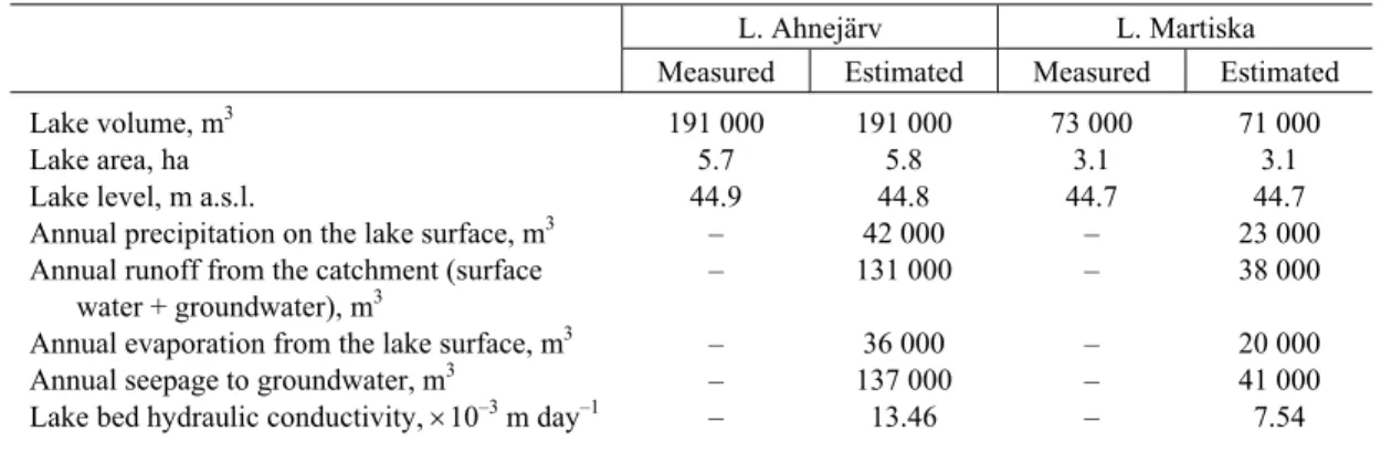
Table 2. Measured and estimated physical properties and water-balance components of L. Ahnejärv and L. Martiska for May 2009. The estimated values were calculated with calibrated lake bed hydraulic conductivities
L. Ahnejärv L. Martiska
Measured Estimated Measured Estimated
Lake volume, m3 191 000 191 000 73 000 71 000
Lake area, ha 5.7 5.8 3.1 3.1
Lake level, m a.s.l. 44.9 44.8 44.7 44.7
Annual precipitation on the lake surface, m3 – 42 000 – 23 000 Annual runoff from the catchment (surface
water + groundwater), m3
– 131 000 – 38 000
Annual evaporation from the lake surface, m3 – 36 000 – 20 000
Annual seepage to groundwater, m3 – 137 000 – 41 000
precipitation on the lake surface. The importance of groundwater seepage from the lake in the annual water-balance outputs from L. Ahnejärv and L. Martiska is 3.8 and 2.0 times (respectively) higher than that of evaporation from the lake surface. This proportion is most probably caused by the drawdown of the Vasavere groundwater abstraction wells. Most of the water in the lumped catchment runoff component presumably originates from groundwater inflow, because the permeable sands surrounding the lake do not favour the formation of surface runoff.
Tool evaluation
To find out how well the tool performs, it needs to be evaluated after calibration with a meteorological dataset from a different time period than the one used for calibration. It would have been better to validate first all the submodels separately against measured evaporation, evapotranspiration, runoff and seepage values from the catchment and only then the complete tool. Unfortunately no such data exist for the catchments and the lakes themselves. Therefore it was only possible to validate the complete tool against the GIS-based lake volume, surface area and water level. But as the equations used in the evaporation and catchment submodels have been extensively verified worldwide (Alley 1984; Dingman 2002; Rushton 2005; Rosenberry et al. 2007; Tao et al. 2007), they were considered to be appropriate for application in our study area.
During the tool evaluation only monthly meteoro-logical inputs were changed and other parameters (including the calibrated hydraulic conductivity) were kept the same as at the end of calibration. Therefore the model needed for evaluation a period with no changes in the hydrological conditions of the lake surroundings. From the available periods of lake level data only one was suitable – from May 2009 to May 2012. The calibrated tool was evaluated using the lake volumes derived from the lake bed DEMs for May 2012 and the monthly meteorological data from June 2009 to May 2012. Lake volumes were derived according to measured lake levels in May 2012, which were 44.9 m a.s.l. (L. Ahnejärv) and 44.3 m a.s.l. (L. Martiska). Lake volumes in May 2009 were taken as a starting point for the evaluation and the monthly meteorological data from the given years were used to drive the evaluation. Finally, the estimated and DEM-based lake volumes from May 2012 were compared with the per cent error statistic acceptable for single-event simulations (Moriasi et al. 2007). The estimated lake volumes in May 2012 were 195 400 and 70 600 m3, respectively, for L. Ahnejärv and L. Martiska; the DEM-based lake volumes at the same time were 190 900 and 60 700 m3, respectively.
The error was therefore 2.4% for L. Ahnejärv and 16.3% for L. Martiska.
To derive margins of error for the complete tool with the calibrated hydraulic conductivity for 2009, a bootstrap approach according to Efron & Tibshirani (1998) was used. The monthly mean precipitation, air temperature, relative humidity, wind speed and cloudiness data from June 1999 to May 2009 were taken as the sampling population. Monthly meteorological data values were drawn randomly with replacement from the sampling population and combined into yearly series. From these randomly generated yearly series only those were retained that had yearly averages (temperature, wind speed, relative humidity) or sums (precipitation) within the actual margins between 1999 and 2009. Altogether 100 different yearly series were derived and used to run the water-balance tool 100 times from an empty lake to equilibration. The standard error (SE) of the water-balance tool with the calibrated hydraulic conductivity for 2009 was derived on the basis of these equilibrium lake volumes.
The SE margins of the tool were ±59 000 m3 for L. Ahnejärv and ±17 000 m3 for L. Martiska. Therefore the estimated lake volumes in 2012 fell well within the limit of 1 SE when compared with the DEM-based lake volumes. Though, the prediction of the volume of L. Ahnejärv was better than the prediction of the volume of L. Martiska.
Simulation design
Three simulations were set up based on precursory knowledge to fulfil the previously stated research objectives.
Simulation 1: Effect of catchment vegetation
The water levels of L. Martiska and L. Ahnejärv dropped from 1946 to 1960 (Fig. 3), and the drop was higher than the annual range of closed-basin water-level fluctuations in the area. According to cartographical and documentary sources, the catchments of the lakes were unforested in 1946, but had been reforested with pines by 1960. Groundwater-altering activities, thus, had not yet started in their vicinity.
63
equilibrium: (a) if the catchments were covered with conifers (Penman–Monteith crop coefficient 1.0 and rooting depth 1.5 m) and (b) if the catchments were covered with moor vegetation (crop coefficient 0.85 and rooting depth 0.3 m). These parameters were taken from Allen et al. (1998). It should be noted that pines grew on the lake catchments in the 1950s, but they were removed from the simulation because of the implementation of the modern analogue.
Simulation 2: Effect of climate
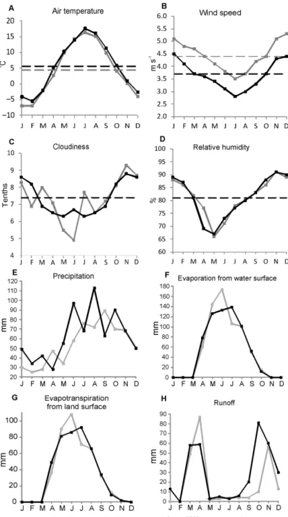
Groundwater abstraction rates were similar at the beginning of the 1970s and at the end of the 2000s, but lake water levels still differed. The average sum of annual precipitation increased in the area from the 1970s to the 2000s, and although annual average air temperature rose as well, wind speed decreased from the 1970s to the 2000s (Fig. 5).
Therefore the question was: ‘Could a climatic shift cause lake-level changes in 30 years?’ The question was answered by using mean monthly values of precipitation, air temperature, wind speed, relative humidity and cloudiness from the 1970s and 2000s as input to the lake evaporation and lake catchment submodel to calculate mean annual evaporation from the lake, precipitation to the lake and runoff from the catchment in the 1970s and 2000s.
Simulation 3: Effect of hydrogeological conditions
The water level of L. Martiska rose by 2.1 m between 1987 and 2009, but only by 1.0 m in L. Ahnejärv. The lakes are so close to each other that changing meteorological conditions affect them in a similar way. Additionally, no significant change in the vegetation cover occurred on the lake catchments during the time period under observation.
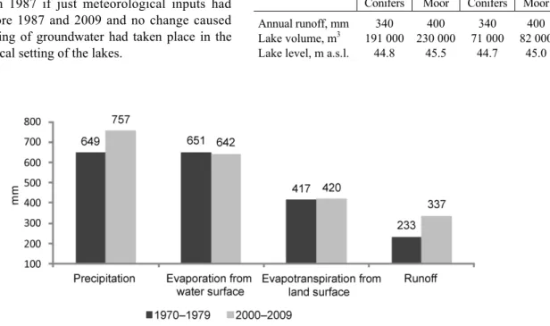
Therefore a third simulation was used to evaluate if the difference in the lake-level rise between 1987 and 2009 at L. Martiska compared to L. Ahnejärv was caused by varying changes in the hydrogeological conditions around the lakes. For that purpose the water balance of the lakes in 1987 was modelled using meteorological inputs from 1977–1986, but leaving hydrogeological inputs, i.e. hydraulic conductivity and catchment area, the same as derived by the calibration run for 2009. The results were compared to actual water level and water volume data corresponding to 1987. Therefore the simulation indicated how high the lake levels would have been in 1987 if just meteorological inputs had differed before 1987 and 2009 and no change caused by the pumping of groundwater had taken place in the hydrogeological setting of the lakes.
RESULTS
Simulation 1: Effect of catchment vegetation
The results showed that if the lake catchments under study were unforested in the present meteorological conditions, annual catchment runoff would be 60 mm, i.e. 18% higher (Table 3). The lakes would contain ~40 000 m3 (L. Ahnejärv) and ~10 000 m3 (L. Martiska) more water. Lake levels would be ~1 m (L. Ahnejärv) and ~0.5 m (L. Martiska) higher.
Simulation 2: Effect of climate
The meteorological data showed that the decadal average relative humidity and cloudiness were alike in the 1970s and the 2000s but other parameters changed significantly. Mean annual precipitation in the 2000s was ~110 mm, i.e. 17% larger, wind speed 0.7 m s–1, i.e. 16% lower and air temperature 1.3°C higher (Fig. 5). The results indicated that these differences caused a ~100 mm, i.e. 43% higher mean annual runoff in the 2000s compared to the 1970s (Fig. 6). Although the mean annual temperature rose from the 1970s to the 2000s, there was no consequent rise of the mean annual evaporation rate. The effect of a higher air temperature
Table 3. Lake volume, level and annual runoff in 2009, estimated with different vegetation on catchments
L. Ahnejärv L. Martiska Conifers Moor Conifers Moor Annual runoff, mm 340 400 340 400 Lake volume, m3 191 000 230 000 71 000 82 000 Lake level, m a.s.l. 44.8 45.5 44.7 45.0
63
was levelled by dropping wind speeds. Mean annual evapotranspiration from the land surface also remained largely the same, additionally bolstering the increase in runoff.
Simulation 3: Effect of hydrogeological conditions
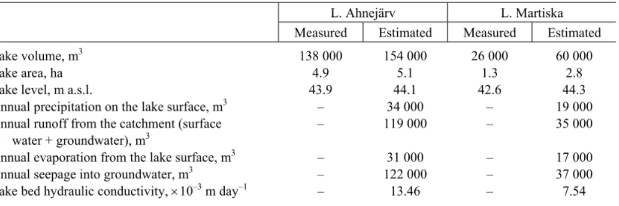
The results showed that if only the precipitation rate, air temperature, humidity and wind speed had changed and the hydrogeological conditions had been the same in the 1980s and in the 2000s, then the water level of L. Ahnejärv would have been almost equal to the level measured in 1987 (Table 4). The water level of L. Martiska, on the contrary, would have been 1.7 m higher. Lake Ahnejärv would have contained ~16 000 m3 and L. Martiska ~34 000 m3 more water in 1987 than they actually did.For L. Martiska the estimated volume was more than two times larger than the measured volume, which would have resulted in a considerably different lake layout (Fig. 7).
DISCUSSION
The first simulation evaluated the effect of vegetation change on the catchments using different crop coefficients and rooting depths for pine forest and moor vegetation. According to the crop coefficients suggested by the Food and Agriculture Organisation, full-grown pine trees are able to evapotranspirate significantly more water than sparse and shallow-rooted moor vegetation (Allen et al. 1998). Consequently, less water that can drain into the lake is left on the catchment. Thus the lake volume decreases and its water level lowers. The simulation suggests that the described phenomenon could have occurred in the study area, as the deforested catchment resulted in water volumes exceeding the actual forested
catchment volumes in 2009 (Table 3). The inter-lake variation is accounted for by differences in the catchment area/lake area ratio, described also in other studies (Harrison et al. 2002; Cardille et al. 2004). Yet, the observed change in water volumes between 1946 and 1960 was significantly larger, 70 000 and 35 000 m3 for L. Ahnejärv and L. Martiska, respectively, than was the addition of water to the lakes in the simulation. In addition to changes in evapotranspiration rates, other processes caused by the removal of forest could exacerbate or mitigate the effect of a change in the evapotranspiration rates. Canopy interception and snowpack accumulation have been described to change considerably after deforestation (Stottlemyer & Troendle 2001), but our data constraints prevented us from simulating these effects.
Even though the simulation considers a different time period than the actual water-level change between 1946 and 1960, we may conclude that, although the additional water from the decreased evapotranspiration caused by the vegetation change would not fully account for the change in the water levels, it still was a contributing factor. The remainder of the change in the water volume from 1946 to 1960 could be explained either by the not simulated processes caused by deforestation or a slight drop in annual precipitation rates registered in more distant meteorological stations in northeastern Estonia (at Narva and Tiirikoja), where data from that period were available (according to data from the EMHI). The lowering of lake level after catchment deforestation has also been described in Calder et al. (1995). More abundant coinciding results exist on analogous changes in river-flows (Twine et al. 2004; Descheemaeker et al. 2006; Siriwardena et al. 2006; Vano et al. 2008). The results, therefore, point out that the vegetation change on lake catchments should be considered as a factor in studies evaluating the causes of both modern and historical lake-level changes.
Table 4. Measured and estimated lake properties and water balance components for 1987, the latter calculated with the hydraulic conductivity calibrated for 2009
L. Ahnejärv L. Martiska
Measured Estimated Measured Estimated
Lake volume, m3 138 000 154 000 26 000 60 000
Lake area, ha 4.9 5.1 1.3 2.8
Lake level, m a.s.l. 43.9 44.1 42.6 44.3
Annual precipitation on the lake surface, m3 – 34 000 – 19 000
Annual runoff from the catchment (surface water + groundwater), m3
– 119 000 – 35 000
Annual evaporation from the lake surface, m3 – 31 000 – 17 000
Annual seepage into groundwater, m3 – 122 000 – 37 000
The most significant water-level drop in the studied lakes coincides well with the initiation of groundwater abstraction. The lowest lake levels were recorded during the years of the highest abstraction (Fig. 2). The subsequent water-level rise, on the other hand, does not fully conform to the reduction of groundwater abstraction. The lake levels were lower in the 1970s than at the end of the 2000s, although groundwater abstraction was basically at the same level. Meteorological data show that the climate in the region became moister, e.g. precipitation amounts rose and wind speed dropped (Fig. 5). The second simulation showed that although the mean air temperature rose, the estimated evaporation rates did not change significantly, because the dropping wind speed reduced the evaporation rate, both from open water and land surface, as saturated air above the surface was not moved away and less water could enter the gas phase (Shuttleworth 1993). Therefore the results suggest that higher water levels in the lakes at the end of the 2000s compared to the 1970s were caused by changes in climate, which brought about higher pre-cipitation and runoff.
Recent climate change has been considered to be the cause of the shrinking area of some large lakes (Abbaspour et al. 2012; Lemoalle et al. 2012) and the change in interannual meteorological conditions the cause of short-term lake-level fluctuations (Mercier et al. 2002; Anda & Varga 2010). The results of the current study, however, indicate that lake-level rise could be taking place in areas where climate is becoming moister. This phenomenon is rarer though, probably because closed-basin lakes, which are most sensitive to changes in climate, are not very common in humid climates (Street-Perrott & Harrison 1985).
63
volume from the measured volume equalling 2 SEs of the tool was recorded, we may conclude that with a 95% confidence level another process affected the water balance of L. Martiska in addition to the change in meteorological conditions. As no vegetation change, except normal maturing of the forests took place on the catchments in 1987–2009, the only other factor influencing the water volume in the lakes could have been a change in the groundwater abstraction rates from the Vasavere wells, which changed some of the hydrogeological properties around the lakes. It has been shown previously that the groundwater level has risen several metres in the region since the beginning of the 1990s when the amounts of groundwater abstraction started to decrease (Häelm 2010). The results of Häelm (2010) also revealed different magnitude of ground-water-level changes in the vicinity of L. Ahnejärv and L. Martiska. The groundwater-level rise has been more significant around L. Martiska which is closer to the wells than L. Ahnejärv. This suits well with the simulation results, as the lake-level rise can be explained by the change in climate at L. Ahnejärv but not at L. Martiska. The larger than estimated groundwater outflow, needed in the third simulation to obtain the measured lake level at L. Martiska in 1987, can therefore be attributed to the effect of a lower groundwater level that would mean a higher lake bed hydraulic conductivity in the tool.
The exact mechanisms of groundwater-level change affecting L. Martiska but not L. Ahnejärv cannot be explained by the simple tool used in this research and need to be studied further with a groundwater flow model and direct measurements of groundwater seepage. Rising groundwater levels could have diminished the previously occurring induced infiltration from the lakes (as described in Sophocleous 2002). However, as the groundwater-level rise has brought about a larger reformation of the local hydrogeological flow system, possibly groundwater catchments and therefore flow directions have also changed. This process is theoretically explained in Winter et al. (1998) and Sophocleous (2002), but respective comprehensive field studies of lakes seem to be lacking.
The results indicate a possibility that one of the underlying assumptions of the water-balance tool – surface-water and groundwater catchments having the same area – is not met and the groundwater component of the tool should be reworked from that perspective. Runoff and groundwater inflow should also be separated in the tool. Still, the simulation results infer that the factors that have caused dramatic water-level fluctuations in L. Martiska and L. Ahnejärv have changed during different time periods and at times different factors
have been functioning simultaneously. For example, the positive trend in lake water-level recovery in 1987–2009 should only partially be explained by the reduction of groundwater abstraction from the Vasavere wells. The recovery was substantially assisted by the natural process of shifting weather conditions. On the other hand, groundwater abstraction cannot account for the entire water-level drop, as before the 1960s the water level fell partly because of the forest that covered the previously unforested lake catchments.
CONCLUSIONS
Poorly documented lake-level changes during a 60-year time-span in two small lakes L. Martiska and L. Ahnejärv were used to make a rough estimation of the varying importance of the role of vegetation, climate and hydro-geology as the causes of these fluctuations. The specific research objectives were evaluated with the help of a spreadsheet-based water-balance simulation tool and the following conclusions were drawn.
– Catchment vegetation change can be an essential factor causing lake-level changes, but in the case of the studied lakes it cannot fully explain the water-level change from 1946 to 1960. Other factors, e.g. climate becoming drier, played a greater role. – Climate change can cause water-level changes in 30
years. In the case of the studied lakes a shift towards moister climate increased the water-balance input components and decreased water-balance output components between 1973 and 2009, causing a higher water inflow to the lakes.
Acknowledgements. This study was supported by the Estonian target-financed project SF0280016s07, Estonian Science Foundation grant MTT3, Environmental Conservation and Environmental Technology R&D Programme Project ‘EDULOOD’ and Doctoral School of Earth Sciences and Ecology. We thank Shinya Sugita for the valuable input concerning the presentation of the simulations, other colleagues from the Institute of Ecology at Tallinn University who read the paper and made constructive amendments, and Donald O. Rosenberry and an anonymous reviewer for helpful comments on the manuscript.
REFERENCES
Abbaspour, M., Javid, A. H., Mirbagheri, S. A., Givi, F. A. & Moghimi, P. 2012. Investigation of lake drying attributed to climate change. International Journal of Environmental Science and Technology, 9, 257–266.
Adrian, R., O’Reilly, C. M., Zagarese, H., Baines, S. B., Hessen, D. O., Keller, W., Livingstone, D. M., Sommaruga, R., Straile, D. & Van Donk, E. 2009. Lakes as sentinels of climate change. Limnology and Oceanography, 54, 2283–2297.
Allen, G. R., Pereira, S. L., Raes, D. & Smith, M. 1998. Crop Evapotranspiration – Guidelines for Computing Crop Water Requirements – FAO Irrigation and Drainage Paper 56. FAO, Rome, 300 pp.
Alley, W. M. 1984. On the treatment of evapotranspiration, soil moisture accounting, and aquifer recharge in monthly water balance models. Water Resources Research, 20, 1137–1149.
Almquist-Jacobson, H. 1995. Lake-level fluctuations at Ljustjärnen, central Sweden and their implications for the Holocene climate of Scandinavia. Palaeogeography, Palaeoclimatology, Palaeoecology, 118, 269–290. Anda, A. & Varga, B. 2010. Analysis of precipitation on Lake
Balaton catchments from 1921 to 2007. Idojaras, 114, 187–201.
Andréassian, V. 2004. Waters and forests: from historical controversy to scientific debate. Journal of Hydrology, 291, 1–27.
Bjerring, R., Olsen, J., Jeppesen, E., Buchardt, B., Heinemeier, J., McGowan, S., Leavitt, P. R., Enevold, R. & Odgaard, B. V. 2013. Climate-driven changes in water level: a decadal scale multi-proxy study recording the 8.2-ka event and ecosystem responses in Lake Sarup (Denmark). Journal of Paleolimnology, 49, 267–285.
Brown, A., Zhang, L., McMahon, T. A., Western, A. W. & Vertessy, R. A. 2005. A review of paired catchment studies for determining changes in water yield resulting from alterations in vegetation. Journal of Hydrology, 310, 28–61.
Calder, I. R., Hall, R. L., Bastable, H. G., Gunston, H. M., Shela, O., Chirwa, A. & Kafundu, R. 1995. The impact of land use change on water resources in sub-Saharan Africa: a modelling study of Lake Malawi. Journal of Hydrology, 170, 123–135.
Cardille, J. A., Coe, M. T. & Vano, J. A. 2004. Impacts of climate variation and catchment area on water balance
and lake hydrologic type in groundwater-dominated systems: a generic lake model. Earth Interactions, 8, 1–24.
Cardille, J. A., Carpenter, S. R., Foley, J. A., Hanson, P. C., Turner, M. G. & Vano, J. A. 2009. Climate change and lakes: estimating sensitivities of water and carbon budgets.
Journal of Geophysical Research: Biogeosciences, 114, G03011.
Davie, T. 2009. Fundamentals of Hydrology. Second Edition. Routledge, London, 200 pp.
Dearing, J. A. 1997. Sedimentary indicators of lake-level changes in the humid temperate zone: a critical review. Journal of Paleolimnology, 18, 1–14.
Descheemaeker, K., Nyssen, J., Poesen, J., Raes, D., Haile, M., Muys, B. & Deckers, S. 2006. Runoff on slopes with restoring vegetation: a case study from the Tigray high-lands, Ethiopia. Journal of Hydrology, 331, 219–241. Digerfeldt, G. 1986. Studies on past lake-level fluctuations. In
Handbook of Holocene Palaeoecology and Palaeo-hydrology (Berglund, B., ed.), pp. 127–144. John Wiley & Sons, New York.
Dingman, S. L. 2002. Physical Hydrology. Second Edition. Prentice Hall, New Jersey, 600 pp.
Efron, B. & Tibshirani, R. J. 1998. An Introduction to the Bootstrap. Chapman & Hall/CRC, New York, 436 pp. [ELB] Estonian Land Board. 1948. Topographical map.
A 1:25 000.
[ELB] Estonian Land Board. 1961. Topographical map. A 1:25 000.
[ELB] Estonian Land Board. 1973. Topographical map. A 1:10 000.
Erg, K. & Ilomets, M. 1989. Mäetööde mõju Kurtna järvede veetasemele – seisund ja prognoos [The effect of mining on the water level of Kurtna lakes – current state and prognosis]. In Kurtna järvestiku looduslik seisund ja selle areng II [Natural Status and Development of Kurtna Lake District II] (Ilomets, M., ed.), pp. 47–54. Valgus, Tallinn [in Estonian].
Fitts, C. R. 2002. Groundwater Science. Academic Press, London, 450 pp.
George, G., Hurley, M. & Hewitt, D. 2007. The impact of climate change on the physical characteristics of the lakes in the English Lake District. Freshwater Biology, 52, 1647–1666.
Gleeson, T., Novakowski, K., Cook, P. G. & Kyser, T. K. 2009. Constraining groundwater discharge in a large watershed: integrated isotopic, hydraulic, and thermal data from the Canadian shield. Water Resources Research, 45, DOI: 10.1029/2008WR007622.
Häelm, M. 2010. Ida-Virumaa pinnaveerežiimi mõjutavad looduslikud ja antropogeensed faktorid Kurtna järvistu ja Purtse jõe näitel [The Influence of Natural and Anthropogenic Factors on the Surface Water Regime According to the Kurtna Lake District and Purtse River (Ida-Viru County)]. MSc thesis, Tallinn University, 60 pp. [in Estonian].
Harrison, S. P., Yu, G. & Vassiljev, J. 2002. Climate changes during the Holocene recorded by lakes from Europe. In
63
Hayashi, M. & Rosenberry, D. O. 2002. Effects of ground water exchange on the hydrology and ecology of surface water. Ground Water, 40, 309–316.
Hostetler, S. W. & Bartlein, P. J. 1990. Simulation of lake evaporation with application to modeling lake level variations of Harney-Malheur Lake, Oregon. Water Resources Research, 26,2603–2612.
Ilomets, M., Paalme, G. & Punning, J.-M. 1987. Kurtna järves-tiku seisund – uurimise eesmärk, strateegia ja võimalu-sed [The state of the Kurtna Lake District – purpose of study, strategy and opportunities]. In Kurtna järvestiku looduslik seisund ja selle areng I [Natural Status and Development of the Kurtna Lake District I] (Ilomets, M., ed.), pp. 8–15. Valgus, Tallinn [in Estonian].
Kaakinen, A., Salonen, V.-P., Artimo, A. & Saraperä, S. 2010. Holocene groundwater table fluctuations in a small perched aquifer inferred from sediment record of Kankaanjärvi, SW Finland. Boreal Environment Research, 15, 58–68. Korhola, A., Vasko, K., Toivonen, H. T. T. & Olander, H. 2002.
Holocene temperature changes in northern Fennoscandia reconstructed from chironomids using Bayesian modelling.
Quaternary Science Reviews, 21, 1841–1860.
Lemoalle, J., Bader, J. C., Leblanc, M. & Sedick, A. 2012. Recent changes in Lake Chad: observations, simulations and management options (1973–2011). Global Planetary Change, 80–81, 247–254.
Linacre, E. T. 1993. Data-sparse estimation of lake evaporation, using a simplified Penman equation. Agricultural and Forest Meteorology, 64, 237–256.
Lode, E., Terasmaa, J., Vainu, M. & Leivits, M. 2012. Basin delineation of small wetlands of Estonia: LiDAR-based case study for Selisoo mire and lakes of Kurtna Kame Field. Estonia. Geographical Studies, 11, 142–167. Mäemets, A. 1977. Eesti NSV järved ja nende kaitse [Lakes of
the Estonian SSR and Their Protection]. Valgus, Tallinn, 263 pp. [in Estonian].
Magny, M., Marguet, A., Chassepot, G. H. & Billaud, Y. 2001. Early and late Holocene water-level fluctuations of Lake Annecy, France: sediment and pollen evidence and climatic implications. Journal of Paleolimnology, 25, 215–227.
Manley, R., Spirovska, M. & Andovska, S. 2008. Water Balance Model of Lake Dojran. BALWOIS 2008, Ohrid, 12 pp. McCabe, G. J. & Markstrom, S. L. 2007. A Monthly
Water-Balance Model Driven by a Graphical User Interface.
http://pubs.usgs.gov/of/2007/1088/pdf/of07-1088_508.pdf, 12 pp. [accessed 01.10.2013].
Mercier, F., Cazenave, A. & Maheu, C. 2002. Interannual lake level fluctuations (1993–1999) in Africa from Topex/ Poseidon: connections with ocean-atmosphere interactions over the Indian Ocean. Global Planetary Change, 32, 141–163.
Moriasi, D. N., Arnold, J. G., Van Liew, M. W., Bingner, R. L., Harmel, R. D. & Veith, T. L. 2007. Model evaluation guidelines for systematic quantification of accuracy in watershed simulations. Transactions of the ASABE, 50, 885–900.
Peńa-Arancibia, J.-L., van Dijk, A. I. J. M., Guerschman, J. P., Mulligan, M., (Sampurno) Bruijnzeel, L. A. & McVicar, T. R. 2012. Detecting changes in streamflow after partial woodland clearing in two large catchments in the seasonal tropics. Journal of Hydrology, 416–417, 60–71.
Penman, H. L. 1948. Natural evaporation from open water, bare soil, and grass. Proceedings of the Royal Society of London, Series A, 193, 120–146.
Perrone, U., Facchinelli, A. & Sacchi, E. 2008. Phosphorus dynamics in a small eutrophic Italian lake. Water, Air & Soil Pollution, 189, 335–351.
Põder, T., Riet, K., Savitski, L., Domanova, N., Metsur, M., Ideon, T., Krapiva, A., Ott, I., Laugaste, R., Mäemets, A., Mäemets, A., Toom, A., Lokk, S., Heinsalu, A., Kaup, E., Künnis, K. & Jagomägi, J. 1996. Mõjutatav keskkond [Affected environment]. In Keskkonnaekspertiis. Kurtna piirkonna tootmisalade mõju järvestiku seisundile [ Environ-mental Assessment. The Effect of Industrial Areas in the Kurtna Region on the Status of the Lakes] (Ideon, T. & Põder, T., eds), pp. 16–48. AS Ideon & Ko, Tallinn [in Estonian].
Punning, J.-M. (ed.). 1994. The Influence of Natural and Anthropogenic Factors on the Development of Land-scapes. The Results of a Comprehensive Study in NE Estonia. Institute of Ecology, Estonian Academy of Sciences, Publication 2, 227 pp.
Punning, J.-M., Koff, T., Kadastik, E. & Mikomägi, A. 2005. Holocene lake level fluctuations recorded in the sediment composition of Lake Juusa, southeastern Estonia. Journal of Paleolimnology, 34, 377–390.
Punning, J.-M., Terasmaa, J. & Vaasma, T. 2006. The impact of lake-level fluctuations on the sediment composition.
Water, Air, & Soil Pollution: Focus, 6, 515–521. Punning, J.-M., Boyle, J. F., Terasmaa, J., Vaasma, T. &
Mikomägi, A. 2007. Changes in lake-sediment structure and composition caused by human impact: repeated studies of Lake Martiska, Estonia. The Holocene, 17, 145–151.
Reta, G. L. 2011. Groundwater and Lake Water Balance of Lake Naivasha Using 3-D Transient Groundwater Model. MSc. Thesis, University of Twente, 54 pp. Rosenberry, D. O., Winter, T. C., Buso, D. C. & Likens, G. E.
2007. Comparison of 15 evaporation methods applied to a small mountain lake in northeastern USA. Journal of Hydrology, 340, 149–166.
Rushton, K. R. 2005. Groundwater Hydrology: Conceptual and Computational Models. John Wiley & Sons Ltd, Chichester, 430 pp.
Shaw, E. M., Beven, K. J., Chappell, N. A. & Lamb, R. 2011.
Hydrology in Practice. Fourth Edition. Spon Press, London & New York, 543 pp.
Shuttleworth, W. J. 1993. Evaporation. In Handbook of Hydrology (Maidment, D. R., ed.-in-chief), pp. 4.1–4.53. McGraw-Hill, New York.
Siriwardena, L., Finlayson, B. L. & McMahon, T. A. 2006. The impact of land use change on catchment hydrology in large catchments: the Comet River, Central Queensland, Australia. Journal of Hydrology, 326, 199–214.
Sophocleous, M. 2002. Interactions between groundwater and surface water: the state of the science. Hydrogeology Journal, 10, 348.
Stottlemyer, R. & Troendle, C. A. 2001. Effect of canopy removal on snowpack quantity and quality, Fraser experimental forest, Colorado. Journal of Hydrology, 245, 165–176.
Street-Perrott, F. A. & Harrison, S. P. 1985. Lake levels and climate reconstruction. In Paleoclimate Analysis and Modeling (Hecht, A. D., ed.), pp. 291–340. John Wiley, New York.
Tamm, T. 2002. Effects of Meteorological Conditions and Water Management on Hydrological Processes in Agricultural Fields: Parametrization and Modeling on Estonian Case Studies. Helsinki University of Technology, Helsinki, 194 pp.
Taner, M. Ü., Carleton, J. N. & Wellman, M. 2011. Integrated model projections of climate change impacts on a North American lake. Ecological Modelling, 222, 3380–3393. Tao, J., Yongqin, D. C., Chong-yu, X., Xiaohong, C., Xi, C. &
Singh, V. P. 2007. Comparison of hydrological impacts of climate change simulated by six hydrological models in the Dongjiang Basin, South China. Journal of Hydrology, 336, 316–333.
Terasmaa, J. 2011. Lake basin development in the Holocene and its impact on the sedimentation dynamics in a small lake (southern Estonia). Estonian Journal of Earth Sciences, 60, 159–171.
Terasmaa, J., Puusepp, L., Marzecová, A., Vandel, E., Vaasma, T. & Koff, T. 2013. Natural and human-induced environ-mental changes in Eastern Europe during the Holocene: a multi-proxy palaeolimnological study of a small Latvian lake in a humid temperate zone. Journal of Paleolimnology, 49, 663–678.
Twine, T. E., Kucharik, C. J. & Foley, J. A. 2004. Effects of land cover change on the energy and water balance of the Mississippi River basin. Journal of Hydrometeorology, 5, 640–655.
Vainu, M. 2011. Häiringute peegeldused järvede veebilansis Kurtna järvistu kolme umbjärve näitel [The Effects of Disturbances on Lake Water-Balance – Based on Three Closed-Basin Lakes in the Kurtna Lake District]. MSc thesis, Tallinn University, 98 pp. [in Estonian].
Valiantzas, J. D. 2006. Simplified version for the Penman evaporation equation using routine weather data. Journal of Hydrology, 331, 690–702.
Vano, J. A., Foley, J. A., Kucharik, C. J. & Coe, M. T. 2008. Controls of climatic variability and land cover on land surface hydrology of northern Wisconsin, USA. Journal of Geophysical Research: Biogeosciences, 113, DOI: 10.1029/2007JG000681.
Vassiljev, J. 2007. Lake level studies: modeling. In Encyclopedia of Quaternary Science (Elias, S. A., ed.-in-chief), pp. 1366– 1374. Elsevier.
Vassiljev, J., Harrison, S. P., Hostetler, P. J. & Bartlein, P. J. 1994. Simulation of long-term thermal characteristics of three Estonian lakes. Journal of Hydrology, 163, 107–123.
Vassiljev, J., Harrison, S. P. & Guiot, J. 1998. Simulating the Holocene lake-level record of Lake Bysjön, southern Sweden. Quaternary Research, 49, 62–71.
Winter, T. C., Harvey, J. W., Franke, O. L. & Alley, W. M. 1998. Ground Water and Surface Water: a Single Resource. Circular 1139, USGS, Denver, Colorado, 79 pp. Yu, G. & Harrison, S. P. 1995. Holocene changes in atmospheric circulation patterns as shown by lake status changes in northern Europe. Boreas, 24, 260–268.
Muutused kliimas, valgla taimkattes ja hüdrogeoloogias kui dramaatiliste veetaseme
kõikumiste põhjused Kurtna järvestikus Kirde-Eestis
Marko Vainu ja Jaanus Terasmaa
Käesoleva uurimuse eesmärk on hinnata, kuidas kliima, valgla taimkate ja hüdrogeoloogilised tingimused põhjusta-vad umbjärvede dramaatilisi tänapäevaseid veetaseme kõikumisi. Näitena on kasutatud Ahnejärve ja Martiska järve Kurtna järvestikus. Püstitatud eesmärgi täitmiseks koostati lihtne MS Exceli-põhine veebilansi hindamise tööriist.