FUNDAÇÃO GETULIO VARGAS ESCOLA DE ECONOMIA DE SÃO PAULO
STEFANIA GREZZANA MERENSTEIN
ESSAYS ON CARTELS AND MARKET DISTORTIONS
FUNDAÇÃO GETULIO VARGAS ESCOLA DE ECONOMIA DE SÃO PAULO
STEFANIA GREZZANA MERENSTEIN
ESSAYS ON CARTELS AND MARKET DISTORTIONS
Tese apresentada à Escola de Economia de São Paulo da Fundação Getulio Vargas como requisito para a obtenção do título de Doutora em Economia.
Área de conhecimento: Organização Industrial Orientador: Vladimir Ponczek
Co-orientador: Paulo Furquim de Azevedo
SÃO PAULO 2016
Grezzana Merenstein, Stefania.
Essays on cartels and market distortions / Stefania Grezzana Merenstein. - 2016.
106 f.
Orientador: Vladimir Pinheiro Ponczek, Paulo Furquim de Azevedo Tese (doutorado) - Escola de Economia de São Paulo.
1. Organização industrial. 2. Concorrência. 3. Cartéis. 4. Combustíveis - Preços. I. Ponczek, Vladimir Pinheiro. II. Azevedo, Paulo Furquim de III. Tese (doutorado) - Escola de Economia de São Paulo. IV. Essays on cartels and market distortions.
STEFANIA GREZZANA MERENSTEIN
ESSAYS ON CARTELS AND MARKET DISTORTIONS
Tese apresentada à Escola de Economia de São Paulo da Fundação Getulio Vargas como requisito para a obtenção do título de Doutora em Economia.
Área de conhecimento: Organização Industrial
Data de Aprovação: 13 de Maio de 2016.
Banca Examinadora:
Prof. Dr. Vladimir Ponczek (Escola de Economia de São Paulo)
Prof. Dr. Bruno Ferman (Escola de Economia de São Paulo)
Prof. Dr. Klenio Barbosa (Escola de Economia de São Paulo)
Prof. Dr. Paulo Furquim de Azevedo (Insper)
Prof. Dr. João Manoel Pinho de Mello (Insper)
AGRADECIMENTOS
Embora esta tese leve apenas o meu nome, tenho a honra de agradecer a ajuda e o apoio de vários indivíduos e instituições que colaboraram para o desenvolvimento deste trabalho ao longo dos últimos quatro anos.
Eu sou grata aos meus orientadores Vladimir Ponczek e Paulo Furquim pelos seus conselhos e recomendações. Eu também gostaria de agradecer aos membros da banca examinadora por suas contribuições. Por último, mas não menos importante, gostaria de manifestar a minha gratidão aos professores do Programa de Pós-Graduação da Escola de Economia de São Paulo por seu papel essencial na minha formação acadêmica.
Faço um reconhecimento especial ao Prof. Luís Cabral, que me guiou e apoiou durante minha estada na New York University Stern School of Business, sem o qual esta tese não teria sido possível, assim como os outros professores nesse departamento e na Universidade de Columbia que contribuíram altamente para a minha formação, me ensinando as ferramentas para a realização deste trabalho.
Agradeço também aos participantes do 43o Encontro da Associação Brasileira de
Pós-Graduação em Economia e aos participantes do Seminário de Tese da Escola de Economia de São Paulo pelos comentários e sugestões.
Gostaria de agradecer aos meus colegas de doutorado e amigos. Tenho imensa gratidão ao meu marido, Ariel Merenstein, que começou e vivenciou esta jornada junto comigo, sua inteligência incomparável foi fundamental para este trabalho de diversas maneiras. Muito obrigado a minha família, especialmente minha mãe Celina Grezzana, pelo eterno apoio. Eu sou muito grata ao meu querido amigo, Rafael Vasconcelos, pela parceria de pesquisa, as discussões intermináveis e, acima de tudo, a amizade incondicional.
Finalmente, agradeço a Fulbright Commission e a CAPES pelo apoio financeiro.
ACKNOLEDGMENTS
Although this dissertation appears to have been completed by one person, I hereby acknowledge the help and support of various individuals and institutions.
I am grateful to my advisors Vladimir Ponczek and Paulo Furquim for their guidance. I would also like to acknowledge the members of the thesis committee for their contributions. Last but not least, I would like to manifest my gratitude to the professors of the Graduate Program from the Sao Paulo School of Economics for their essential role in my academic formation.
A special appreciation to Luis Cabral, who guided and supported me during my period at the New York University Stern School of Business without whom this thesis would not have been possible, as well as the other professors in that department and at Columbia University who contributed highly to my formation teaching me the tools to accomplish this work.
I also thank seminar participation at the 43th Meeting of the Brazilian Association of Graduate Programs in Economics and the Thesis Seminars of Sao Paulo School of Economics for helpful comments and suggestions.
I would like to thank my graduate school colleagues and my friends. My gratitude also goes to my husband, Ariel Merenstein, who started and lived through this journey with me, your unparalleled intelligence was fundamental to this work on so many levels. Many thanks to my family, especially my mother Celina Grezzana, for the everlasting support. I am very grateful to my dear friend, Rafael Vasconcelos, for the research partnership, the endless discussions and above all the unconditional friendship.
ABSTRACT
This dissertation is a conjunction of three essays on the Industrial Organization field, this empirical work is applied to the Brazilian retail gasoline market. The first essay investigates the existence of spillover effects from cartel activity. The second essay relates the well-known economic puzzle of asymmetric cost pass through to prices with the existence of horizontal coordination - cartels - in the relevant market. Finally, the third essay investigates the effectiveness of antitrust interventions inside the offenders and the consequences of its disclosure in related markets.
Keywords: Cartel, Cartel Spillover, Cost Pass Through Asymmetry, Disclosure of Antitrust Enforcements.
JEL Classification: D22, L11, L41, L44 , L81.
RESUMO
Esta tese é uma conjunção de três ensaios sobre no campo de organização industrial, o trabalho empírico é aplicado ao mercado brasileiro de revenda de combustíveis, especificamente gasolina. O primeiro ensaio investiga a existência de efeitos indiretos, repercussões para outros mercados, resultantes da atividade do cartel. O segundo ensaio relaciona o conhecido tema da literatura de repasse assimétrico de custos aos preços com a existência de coordenação horizontal - cartéis - nos mercados em questão. Finalmente, o terceiro ensaio investiga a eficácia das intervenções de defesa da concorrência dentre os infractores e as consequências da sua divulgação em mercados relacionados.
CONTENTS
Agradecimentos vi
Acknoledgments vii
Abstract viii
Resumo ix
List of Figures xii
List of Tables xiii
Chapter 1. Introduction 1
Chapter 2. Cartel Spillover: the effect of cartel proximity on pricing behavior 3
1 Introduction 3
2 The Data and The Market 5
3 Measuring the Impact of Cartel Spillover 13
4 Conclusion 19
5 Appendix 23
Chapter 3. Cost Pass Through: Does collusion potentiate price asymmetry? 32
1 Introduction 32
2 The Data and The Market 35
3 Measuring the Asymmetry on Cost Pass Through 41
4 Conclusion 51
5 Appendix 52
Chapter 4. Public Displayed vs. Private Enclosed: The Effect of the Publicization of
Antitrust Enforcements 57
1 Introduction 57
2 Data 64
3 Measuring the Effect of the Publicization of Antitrust Enforcements 70
4 Conclusion 83
5 Appendix 86
LIST OF FIGURES
2.1 Price Distributions Before and During cartel Activity 13
2.2 Evolution of prices and costs for Cartelized stations 23
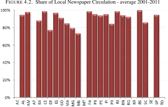
3.1 Average prices and costs for the Retail Gasoline Market 39 3.2 Average prices and costs for the Retail Gasoline Market for Cartel Members 39 4.1 Result from the cases analyzed in the study, by type of Intervention 59 4.2 Share of Local Newspaper Circulation - average 2001-2011 60 4.3 Price Levels after an Antitrust Enforcement, by type of Intervention 76 4.4 Price Margins after an Antitrust Enforcement, by type of Intervention 77 4.5 Price Variance After an Antitrust Enforcement, by type of Intervention 78 4.6 Price Levels Before an Antitrust Enforcement, by type of Interventiont 81 4.7 Price Margins Before an Antitrust Enforcement, by type of Intervention 83 4.8 Price Variances Before an Antitrust Enforcement, by type of Intervention 84
4.9 Types of Interventions 86
LIST OF TABLES
2.1 Descriptive Statistics 10
2.2 Descriptive Statistics - On and Off Cartel 12
2.3 Effect of a Cartel onset for Cartel Members and other Submarkets, Simple Difference 15 2.4 Effect of a Cartel on Price Levels, Margins and Variance 17 2.5 Tests of the difference in coefficients for the Effect of a Cartel 18 2.6 Robustness Check: Effect of a Cartel on Price Levels, Margins and Variance 20 2.7 Robustness Check: Tests of the difference in coefficients for the Effect of a Cartel 21 2.8 Effect of a Cartel on Price Levels, Margins and Variance (complete) 25 2.9 Robustness Check: Effect of a Cartel on Price Levels, Margins and Variance (complete) 26
3.1 Descriptive Statistics 40
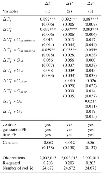
3.2 Change in Prices and Costs for Cartel Members and Non-Members 41
3.3 Estimates of Cost Pass Through 43
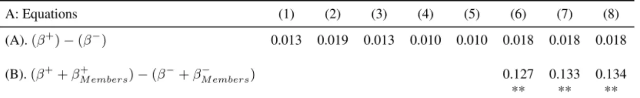
3.4 Test of Difference Between the Sum of Coefficients 43
3.5 Estimates of Cost Pass Through, Extended Reach Market 44
3.6 Test of Difference Between the Sum of Coefficients, Extended Reach Market 45 3.7 Estimates of Cost Pass Through, Longer Adjustment Period 47 3.8 Test of Difference Between the Sum of Coefficients, Longer Adjustment Period 48 3.9 Probability of Price Change given the Cartel Agreement 49 3.10Probability of Price Change given the Last Digit of Prices 49 3.11Probability of Cartel Agreement given the Last Digit of Prices 50
3.12Estimates of Cost Pass Through (complete) 52
4.1 Descriptive Statistics 69
4.2 Descriptive Statistics, by type of Intervention 71
4.3 Effect of an Antitrust Enforcement 26 weeks following an Intervention 74 4.4 After an Antitrust Enforcement, by type of Intervention 79 4.5 Before an Antitrust Enforcement, by type of Intervention 82 4.6 Effect of an Antitrust Enforcement 26 weeks following an Intervention (complete) 87 4.7 Effect of an Antitrust Enforcement 13 weeks following an Intervention (complete) 88 4.8 Effect of an Antitrust Enforcement 52 weeks following an Intervention (complete) 89 4.9 After an Antitrust Enforcement, by type of Intervention (complete) 90 4.10Before an Antitrust Enforcement, by type of Intervention (complete) 96
CHAPTER 1
INTRODUCTION
The economic literature have extensively studied cartel agreements, how to prevent them, how to screen and uncover them, how players actually sustain them. By and large, the obstruction of competition caused by collusive agreements are seen as damaged to consumers and as such are condemned by the competition authorities around the globe as a condemnation
per se, that is, if there is proof, no investigation is required, the condemnation is straightforward.
Nonetheless, cartels are still everywhere pervading the competitive market context. The Brazilian antitrust agency have put a lot of effort into investigating and punishing cartels since the mid-2000s, attacking the main source of complaints by consumers. More than 20% of the complaints that arrive at the agency are related to cartel activity or the suspicion of such and the retail gasoline market is by far the industry most called upon.
This dissertation is a conjunction of three essays on the Industrial Organization field which we seek to study cartels and its consequences to the competitive environment where they operate, pointing out market distortions yield by its activity. However, we do not focus solely on the competitors that actually engaged in the offense. We attempt to look at its consequence in a broader spacial range.
however, is limited to firms that compete in the same market. It does not spread out to stations located in nearby cities, which means that mutual distributors and commuters are insufficient to generate any spillover effect of the cartel. The result is a direct effect from the Bertrand competition model that predicts that firms taking part in the cartel set prices taking into account their competitors strategies and have no incentive to deviate when playing an infinite Bertrand game. Players in the vicinity - even if out of the cartel agreement - have no incentive to charge prices equal to marginal cost either as they can have higher profit by charging just below the cartel price. Thus, our results corroborate the common definition of the municipality as the relevant market for the retail gasoline market.
Chapter 3 addresses a well-known puzzle in the economic literature that is the asymmetry of cost pass through to prices. The empirical literature seem to contradict the classical theoretical one, since the later states that prices should move symmetrically to accommodate cost increases or decreases. In chapter 3 we provide an explanation for such asymmetry based on the existence of cartel agreements preventing prices to move symmetrically. The knowledge of cartel activity allows us to isolate price asymmetric behavior in cartelized from non-cartelized markets and our results conclusively indicate that collusive agreements are responsible for the asymmetry of cost pass through. We find strong evidence that retailers under collusion refrain from cutting prices in response to a decrease in costs and would instead rely on current existing prices as a focal point for coordination.
Following, in chapter 4, we assess the importance of antitrust enforcements as a deterrence mechanism to future cartel-like prices. In fact, we go even further appraising the relevance of the disclosure of the antitrust action among the offenders and also its spillover effects to other submarkets. We look at firms that actively took part on cartel agreements as well as related markets and investigate if firms react differently to publicly disclosed (dawn raids) as oppose to private enclose (mail notifications) antitrust enforcements. We find that the deterrence effect of a publicly displayed antitrust intervention is higher and immediate for the indicted stations but it is also present among stations located in the same municipality and nearby cities that did not partake on the offense. Additionally, stations seem to not care at all about the receipt of a mail notification. We conclude that the public display of an intervention seem to have an important role in preventing future cartel-like price behavior not only among offenders but also to set an example to other possible offenders.
Finally, we present the conclusions for this dissertation in chapter 5.
CHAPTER 2
CARTEL SPILLOVER: THE EFFECT OF CARTEL PROXIMITY ON PRICING
BEHAVIOR
Abstract
By studying the onset of cartels, we intend to test and quantify the impact of cartel agreements on pricing pattern not only within its members but also among players outside the collusive agreement. Using a large dataset from the Brazilian retail gasoline market, we look at pricing behavior amid firms that actively took part on cartel agreements as well as related markets. Our results indicate that by interacting directly with firms that are under a cartel agreement, non-collusive firms also increase the magnitude of their prices as a result of direct Bertrand competition. The spillover effect from the cartel, however, is limited to firms that compete in the same market: mutual distributors and commuters are insufficient to generate any spillover effect of the cartel. Our results also corroborate the common definition of the municipality as the relevant market for the retail gasoline market.
1 Introduction
Collusive agreements have long been studied and pointed out as damaged to consumers. The Brazilian antitrust agency have put a lot of effort into investigating and punishing cartels since the mid-2000s, attacking the main source of complaints by consumers. More than 20% of the complaints that arrive at the agency are related to cartel activity or the suspicion of one and the retail gasoline market is by far the industry most called upon.
they create incentives to sustain the agreement. In addition, influential theoretical and empirical studies from Porter [1983], Green and Porter [1984], Rotemberg and Saloner [1986] and Ellison [1994] have shown that large demand shocks impact cartel stability, duration and eventually can lead to price wars. Yet, little is known about cartel’s development to related markets.
Our objective in this paper is to quantify the impact of cartel agreements on pricing not only within, but also outside the collusive agreement by studying the onset of cartels. In order to address our basic research question, we analyze data from the Brazilian retail gasoline market. Our data includes retail and distribution prices at the retail pump level for a large sample of gasoline stations across Brazil’s territory, from July 2001 to December 2011. During this period, many cases of cartel were uncovered, therefore, active during this period.
In Brazil, retail gasoline prices are publicly displayed by law. The objective of this regulation is to facilitate consumers’ search and prevent horizontal coordination. However, the rule is faulty. If in the one hand it facilitates consumer search, in the other hand it also serves as an information mechanism for cartel members to oversee the maintenance of the agreement. The fact that undercutting is almost immediate, retaliation is instantaneous so it is more costly to firms to incur in price cutting behavior, making collusion easier to sustain. It also favors competitors strategy setting, when they are, in fact, competing.
Considering gasoline a homogeneous product and firms setting prices taking into account an infinite Bertrand game, cartel members have no incentive to deviate so they play the cartel (monopoly) price. In the meantime, players in the vicinity - even if out of the cartel agreement - have no incentive to charge prices equal to marginal cost either as they can have higher profit by charging just below the cartel price. In this scenario, the cartel agreements have impact not only on cartel members, but also on firms in its relevant market.
In this study we want to test the existence of this spillover effect from the cartel and, if existent, how far does it spread out. The above rationing is straight forward for stations in the proximity of a cartel. Yet if we consider commuters and information passed along by distributors, the effect of the cartel could be extrapolated to other related stations, causing the cartel to have larger spillover effects. Whilst there are many paper studying cartels, and even the effect of spillover from antitrust enforcements (Block and Feinstein [1986]), to the extent of my acknowledge the spillover from the cartel activity has not been a topic of extensive study.
In the first part of the paper, we present the data and document the existence of a high retail pricing pattern among cartels members. We corroborate the literature finding that the typical feature of cartel behavior is to increase prices and margins, as well as to reduce price variance.
Moreover, over the same period, we show that the higher prices and margins are not limited to the cartel members but pass along to the other gas stations operating in the same market (same municipality).
In the second part of the paper, we quantify the cartel effect whilst simultaneously testing the existence of a spillover effect of the cartel on other markets.
Our results indicate that the spillover effect is restricted to stations inside the same municipalities where the cartel took place, which confirm the result of the Bertrand game and also the common definition of relevant market for the retail gasoline as the municipality. No spillover effect was found among stations in nearby municipalities or elsewhere in the State indicating that commuters and distributors are insufficient to influence the competitive equilibrium of these markets.
2 The Data and The Market
The data used in this analysis comes from a weekly price survey conducted by the Brazilian National Petroleum Agency (ANP, at the Brazilian acronym) calledSistema de Levantamento de Preços (SLP). The agency surveys a sample of stations throughout the Brazilian territory
in order to monitor prices, covering 555 municipalities in Brazil, approximately 10% of the municipalities in the country1. Our data comprises weekly data from July 2001 through
December 2011 (548 weeks).
The data corresponds to weekly gasoline prices at the gas-station level. Not all stations are audited on a weekly basis, in fact the number of gas stations audited each week is previously determined. The assortment of stations that will be audited each week is randomly assigned by the Brazilian national agency, making the dataset an unbalanced panel. Note that the station’s employees have no knowledge about which gas stations have been assigned until the agency’s technician is at the designated stations.
It is important to mention that during the analyzed period sixteen cases of cartel activity were uncovered in Brazil. Most were investigated by CADE (the Brazilian antitrust authority) because of a previous criminal investigation by the local prosecutor authority. There has been evidence of anti-competitive activity in Bauru (SP), the metropolitan area of Belo Horizonte (MG), Caxias do Sul (RS), Cuiabá and Várzea Grande (MT), Goiânia (GO), Guaporé (RS), João Pessoa (PB), Lages (SC), the metropolitan area of Londrina (PR), Manaus (AM), Natal (RN), the metropolitan area of Recife (PE), Santa Maria (RS), Teresina (PI) and the metropolitan area
of Vitória (ES). These cases were uncovered and then analyzed and in most cases condemned by CADE2.
Among 5,285,052 observations compiled, 5,244,340 (99.23%)3reported prices for gasoline.
Prices are reported in the national currency, the Reais. These gas stations had their prices measured during 548 weeks (Jul/2001 through Dec/2011), covering on average 9,983.79 gas stations per week (minimum of 1 and maximum of 12,685) and 555 municipalities, with 31,555 gas stations overall in the sample, 1,817 of which were part of a cartel at some point in time. Each municipality had on average 66.52 gas stations audited each week (minimum of 1 and maximum of 840), although that varies according to the size of the municipality as well as the time within the survey. In the beginning, the survey had a much smaller scale than it has in the more recent period.
The dataset contains information on prices of retail and acquisition of gasoline for each gas station sampled. We will take the prices of which the retailer buys gasoline from the distributor (the acquisition price) as a proxy for costs. We understand that there are many other costs related to the operation of a gas station such as labor and rent but we believe this is the main cost. In fact, this price represents, on average, 85.7% of the retail price (as indicated by table 2.1). That is, with the acquisition price even if we do not know the exact cost function of the firm we have the single most important variable cost of the business which is the price with which the establishment acquires its main retail product. The cost data is not reported for every single data entry. In this sample, 62.88% of the gas stations reported the price with which they acquired the gasoline they were retailing4. From now on this price will be referred as the
acquisition price.
The data also contains information on its location/address, company owner, and brand in the case that the station is not independent and has a distributor associated with it. We paired this dataset with the ANP registry of operating gas stations as a way to establish when this gas station started/end its activity, so that we could compute the total number of gas stations operating in each market. This pairing was also important to allow us to correct the stations identifications, so we could follow the firm throughout the years. In fact, this is what makes this dataset so unique. Whilst other studies use the same source of data, they either use the
2Goiania (GO) and Cuiabá and Várzea Grande (MT) were dismissed because of evidence contamination; João
Pessoa (PB), Natal (RN) and the metropolitan area of Belo Horizonte (MG) are still under investigation. In all cases we consider the existence of the cartel because records of phone calls or documents give us strong belief that there was a cartel operating in that market, and if the antitrust agency is unable to condemn the defendant, is due to some judicial stratagem, that is, the cases were not dismissed on merits but on formal grounds.
30.77% are missing data.
4There is a topic in the literature arguing that there is an upper bias in the report of acquisition prices of gasoline,
pointing out that the stations that do not report are the ones paying the least. This would cause us to underestimate the price margin as well as all estimates associated with it.
data as cross sections, or they use it as panel data but aggregated by municipality. We, on the other hand, worked the raw data to be able to use it at the station-level and also in the panel configuration, fixing each data entry’s identification and address according to ANP’s registry.
Finally, we obtain detailed information on each cartel case, including participants and relevant dates, through the court files. We have the information of when, precisely, each gas stations suffered an antitrust intervention and we will consider this the ending date of the corresponding cartel. For the onset of the cartels, however, we use the earliest record of a meeting or conversation between members, live or by phone, suggesting a price-fixing deal that the lawsuit has records of. The period between these two dates will be considered the duration time of each cartel for the purpose of this study. All other time periods will be considered off cartel.
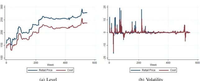
Figure 2.2 in the appendix presents the evolution of prices and costs for each municipality where there has been a cartel case. To construct this figures we took the average of prices and costs across all stations that took part in the cartel. The vertical lines are selected based on information from the court documents. The solid red line is the date when the authority intervened in the cartel, we assign this date as the end of the cartel. The dashed red line is the first reported date of cartel activity according to the authority’s records. However, in our empirical exercises, we also consider a few different longer windows of cartel activity extending the initial date 4, 13 and 26 weeks pre-records - the equivalent of 1, 3 and 6 months, respectively. In this study we focus our attention on the gas stations that were part of the collusive agreement, and stations geographically connected to them. We consider the connection to be stronger the closer the station is to the core of the cartel owing to the fact that retail gasoline prices are publicly displayed so consumers (locals and commuters) can easily search prices and purchase accordingly, but also due to sharing the same distributors, who may facilitate the flow of information between stations, be it voluntarily or at the request of retailers. These stations are observed for a large number of consecutive periods - despite the attrition - and experience the same aggregate demand and cost shocks.
In what follows we will describe the variables that will be used as well as provide some descriptive statistics of the sample.
2.1 Dependent Variables
(we construct the price margin variable using ourCost variable which we will describe in the
following subsection) and price variance.
We also deflated all prices, that is, the retail and the acquisition prices. On the one hand, Brazilian retail gasoline prices do not follow market inflation directly since they are controlled by the government, this is also why crude oil prices cannot be used as a predictor of gasoline prices in Brazil. On the other hand, we will be comparing different time periods, that is, period with and without cartels, that are largely diffused along the over 10 years dataset we use.
Brazil has a long history of high inflation and from July 2001 to December 2011 inflation was up to 80% in the consumer’s prices index (IPCA, for the Brazilian index). Prices of retail and acquisition of gasoline increased during this period 65.6% and 63.2%, respectively.
Although we do not have data all the way through 2015, we deflated prices to September 2015 so that the magnitudes of the effects are up to date, during which inflation accumulated an increase of 152% (from July 2001 to September 2015).
2.2 Independent Variables
We use the information contained in the court documents as well as other information contained in the ANP data to create other relevant variables. We construct statistics on a weekly basis, so we have information varying on periods before and after the implementation of the cartel agreements.
For instance, we take the name of the defendants in each of the civil actions and we used this information to create a dummy variable that define the group of stations that participated in each of the collusive agreements -�M embers -, that is, the cartel members. There are cases in which the union of gas stations was responsible for organizing and enforcing the cartel and, in that case, we appointed as members of the cartel all gas stations that were part of the union at the time of the cartel activity5.
We then compute three other dummies to define the other geographic variables of interest which are all complementary to each other, such as: the variable�M includes all gas stations located inside the market where the cartel took place - it can be one or more municipalities - but that were out of the cartel agreement. These firms, expressed by the�M variable, are the ones with the highest proximity to the collusive market. If there is indeed a spillover effect from the cartel activity, these firms should capture the highest influence from the cartel without actually participating in it.
5We obtained this information on the lawsuits through the list of gas stations affiliated to the union at the time of
cartel operation.
Following, we compute the �M sr variable. The �M sr includes the gas stations that are located in the same mesoregion6as where the cartel took place, that is, all gas stations located in
nearby cities. We exclude the gas stations that are part of�M embersor�M. Lastly, we compute the�S variable which includes the gas stations that are located in the same State7where the cartel took place excluding the gas stations that are part of�M embersor�M or�M sr. Succinctly, all stations located inside a State where a cartel took place will integrate one, and only one, of these four variables/groups depending on their geographical proximity to the collusive market.
Although, the gas stations included in�M sr and�S are not directly connected to the cartel firms since they are not even in the same municipality, we include them in our estimation to test the hypothesis of how far does it go the spillover effect of the cartel. After all, they are supplied mostly by the same distributors and also commuters may arbitrage these markets.
We also use the information contained in the lawsuits to estimate an approximate date of cartel beginning; based on the records of a meeting between members, a phone call to fix prices, etc. We do understand that the assignment of this date is less precise than the cartel ending, this is why our main estimations do not consider the period before the first date mentioned in the court files as control variables at all. As a robustness check to our results we test different dates and control groups to make sure the omission of the exact date of cartel beginning do not compromise our results8.
We use the information in the ANP data to construct our outcome variables as well as measures of market structure at the municipality level. Specifically, we are interested in measuring the total number of stations and the share of low branded or independent selling stations9. We also construct measures of market structure in the gas station level such as:
dummies indicating the location of the gas station, i.e., if in a street, avenue, highway or secondary road; a dummy variable indicating if the gas station is branded10 and dummies
indicating the eleven main brands operating nationally11.
6A mesoregion is a subdivision of the Brazilian states, grouping together various municipalities in proximity and
with common characteristics.
7Brazil is a federation composed by 26 states plus the Federal District.
8The cartel activity could have started before the dates reveled in the court files. In that case, the resulting control
period has higher average prices than it would if we knew the accurate commencement dates. Although not ideal, this problem seems less important here because it would play against our results by weakening them.
9All brands except the ones that are part of Sindicom - the national union of fuel distributors - are considered
low brand stations in the context of this work, that means high branded are the ones associated to Sindicom and independent stations are brand-less stations.
10The variable equal 1 to the gas stations that have any sort of brand associated with it and 0 to the independent
stations.
11These 11 dummies comprehend Ale, Air BP, BR Petrobras, Ipiranga, Chevron, Cosan, Esso, Repsol, Shell,
Finally, we include as a control variable the marginal cost which is represented by theCost
variable. Considering only 62.88% of the stations in the sample reported the acquisition price, we input the weekly average of each municipality for the remaining stations. If no station in that municipality reported an acquisition price for that week a missing value is assigned to that entry. This could happen especially in small municipalities where fewer gas stations are audited each week. We use thisCostvariable to compute our margin outcome variable.
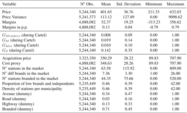
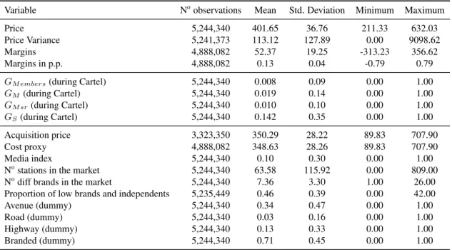
Table 2.1 provides descriptive statistics on the above mentioned variables for the whole sample, whilst in table 2.2 we break down by on and off cartel activity for the subsample of stations that ever participated in the offense and stations with geographical proximity to them. The average price throughout the sampled period considering prices deflated for September 2015 is 401.65 cents, with 52.37 cents of which being the retailer margin, that is 13% of its revenues12.
TABLE 2.1. Descriptive Statistics
Variable NoObs. Mean Std. Deviation Minimum Maximum
Price 5,244,340 401.65 36.76 211.33 632.03
Price Variance 5,241,373 113.12 127.89 0.00 9098.62
Margins 4,888,082 52.37 19.25 -313.23 356.62
Margins in p.p. 4,888,082 0.13 0.04 -0.79 0.79
GM embers(during Cartel) 5,244,340 0.008 0.09 0.00 1.00
GM(during Cartel) 5,244,340 0.019 0.14 0.00 1.00
GM sr(during Cartel) 5,244,340 0.010 0.10 0.00 1.00
GS(during Cartel) 5,244,340 0.142 0.35 0.00 1.00
Acquisition price 3,323,350 350.29 28.22 89.83 707.90
Cost proxy 4,888,082 348.63 28.26 89.83 707.90
Nostations in the market 5,244,340 63.58 115.92 0.00 809.00
Nodiff brands in the market 5,244,340 7.36 3.30 1.00 26.00
Nostations branded in the market 5,244,340 44.35 75.66 0.00 520.00
Proportion of low brands and independents 5,235,449 0.46 0.39 0.00 42.00
Density of stations per municipality 5,235,449 0.46 0.39 0.00 42.00
Avenue (dummy) 5,244,340 0.34 0.47 0.00 1.00
Road (dummy 5,244,340 0.03 0.16 0.00 1.00
Highway (dummy) 5,244,340 0.13 0.33 0.00 1.00
Branded (dummy) 5,244,340 0.71 0.45 0.00 1.00
Note: All currency figures are in cents of Reais deflated for September 2015. Data are from 555 municipalities in Brazil from 2001:7 - 2011:12 at the station-level on weekly basis.
Following we have each group variable (dummies). What calls our attention the most is the fact that�M (during cartel) is almost twice the size of�M sr (during cartel), 1.87% versus 1.05% respectively, even though�M sr includes a much larger group of municipalities. This is not surprising though, as we note that the municipalities where there were cartel agreements are big cities (the biggest in their corresponding mesoregion) and so they include a higher number
12Note that this is margins before fixed costs.
of stations. �M embers (during cartel) represent only 0.85% of the sample points, although it is not little when we consider it is 44,471 observation points.
Among the control variables we observe that, by construction, the number of observations among theCostvariable is higher than theAcquisition price. As a result of our data imputation
we allowed an extra 1,564,732 observations to be used. There are on average 63.58 gas stations per municipality and 7.36 different brands. A significant 45.6% of the stations are of low brands or independent, that is, they are not part of a major gasoline brand. Just over 50% of the stations are situated at streets (the base variable), followed by avenues with 34% and main roads and highways with 13%. Approximately 30% of the market is constituted by independent stations, as 70% are branded by either a high or low brand. Independent stations are known to increase competition as they usually sell with lower retail prices, as shown by Hastings [2004]. The objection is that they tend to sell lower quality fuel.
Table 2.2 displays the descriptive statistics for the period before and during the cartel operation. As mentioned previously, cartels happened in different times throughout the ten years analyzed, so the length of both periods, on and off cartel, are different for each cartel. Table 2.2 also contains information on the outcome variables for the other submarkets.
Analyzing Panel A, we observe that the average price and margins are substantially higher for stations during the cartel operation. Prices are, on average,38cents of Reais higher during
the agreement than off of it. Interesting to notice, though, that not all price increment is converted into margin expansions as costs are also higher during the cartelized period. Still margins are a staggering24cents higher which implies in an increment of over50%in margins.
The fact that costs are higher (not statistically) during the period of cartel operation alludes to the discussion that cartel’s emergence are endogenous and linked to a tougher market environment. With respect to the other submarkets (Panels B, C and D), we observe that prices and margins are higher for stations inside the municipality where the cartel took place and the municipalities nearby (mesoregions), the opposite is true for stations located elsewhere in the same State.
2.3 Comparing Gasoline Prices Before and During Cartel Activity
Following table 2.2, we show in this subsection price changes that occurred before and during cartel activity for cartel members and stations inside the same municipalities.
TABLE 2.2. Descriptive Statistics - On and Off Cartel
Off (Before) On (during)
Variable NoObs. Mean Std. Deviation NoObs. Mean Std. Deviation
Panel A. Stations from theGM embersgroup
Price 22,748 405.05 31.97 43,349 443.18 42.95
Price Variance 22,575 87.42 134.53 43,072 82.90 178.56
Margins 22,738 50.09 21.30 42,566 74.34 23.97
Margins in p.p. 22,738 0.12 0.05 42,566 0.16 0.04
Acquisition price 17,972 355.84 24.47 30,836 370.69 26.10
Cost proxy 22,738 354.95 24.52 42,566 369.62 27.05
Nostations in the market 22,748 78.95 68.95 43,349 53.77 26.91
Nodiff brands in the market 22,748 8.97 1.92 43,349 7.36 2.17
Nostations branded in the market 22,748 67.17 59.89 43,349 35.10 25.04
Proportion of low brands and independents 22,748 0.29 0.17 43,349 0.57 0.30
Density of stations per municipality 22,748 0.30 0.21 43,349 0.10 0.15
Avenue (dummy) 22,748 0.62 0.48 43,349 0.66 0.47
Road (dummy 22,748 0.01 0.10 43,349 0.01 0.11
Highway (dummy) 22,748 0.09 0.28 43,349 0.10 0.30
Branded (dummy) 22,748 0.89 0.32 43,349 0.64 0.48
Panel B. Stations from theGM group
Price 123,763 397.01 31.29 92,736 407.64 37.07
Price Variance 123,762 113.12 104.37 92,699 97.75 147.97
Margins 123,598 43.33 19.65 89,446 53.36 20.34
Margins in p.p. 123,598 0.11 0.04 89,446 0.13 0.04
Panel C. Stations from theGM srgroup
Price 38,319 408.34 27.54 52,957 419.89 35.32
Price Variance 38,317 75.99 102.13 52,955 85.16 146.67
Margins 37,268 55.07 16.86 49,588 59.51 20.02
Margins in p.p. 37,268 0.13 0.04 49,588 0.14 0.04
Panel D. Stations from theGSgroup
Price 247,961 417.18 27.18 742,162 413.36 35.67
Price Variance 247,951 72.39 104.63 742,148 116.25 137.39
Margins 233,203 59.01 17.20 712,044 54.27 19.56
Margins in p.p. 233,203 0.14 0.04 712,044 0.13 0.04
Note: All currency figures are in cents of Reais deflated for September 2015. Data are from 555 municipalities in Brazil from 2001:7 - 2011:12 at the station-level on weekly basis. We exclude cities, mesoregions and States with multiple cartels during the sampled period because the definition of before and during (on and off) would be compromised.
same municipality but out of the cartel agreement, in subfigure (b). We observe a staggering shift among cartel members, but we also observe a small movement in the distribution of prices of the other stations inside the same municipality. In subfigure (c) we observe that even before the cartel implementation, the stations that never took part in the cartel were charging prices slightly below the ones that later would come to commit the offense.
We also perform mean tests comparing prices before and after (as seen on table 2.2) for each group of stations as well as across them and we find average prices to be consistently different over time (before and after the cartel implementation) and also over groups of stations.
FIGURE 2.1. Price Distributions Before and During cartel Activity
(a) Cartel Members (b) Stations inside the municipality
(c) Before cartel activity (d) During cartel activity
All figures are in cents of Reais. Data are from 555 municipalities in Brazil from 2001:7 - 2011:12 at the station-level on weekly basis. Weekly averages are taken across all gas stations.
3 Measuring the Impact of Cartel Spillover
Our objective in this paper is to quantify the impact of cartel spillover and implicit information on retail price levels, margins and price variance. We do so by evaluating these outcome variables on and off (before) cartel periods, and within submarkets with geographical proximity to the cartelized market. We label this the indirect effect of cartel agreements.
There is no legal evidence of price coordination outside the stations directly involved in the offense and the fact that station ownership in Brazil is typically local, in addition to the separation of ownership between gasoline producers and retailers, allows us to measure the spillover effect more accurately than in markets where production and retailing of gasoline are owned by the same players, or when one or more players in one market have high insertion in other markets.
separately13. Following, we have our main estimation, subsection 3.2 where we test all
submarkets together. In both cases we discard the observations for the period before the cartel allegedly started.
Allegedly, because this is the first record of a meeting or a phone call on the court documents, but it does not necessarily mean that the cartel was not operating before that without the knowledge of the authorities. Considering the period before this set date could be contaminated by cartel activity, we discard it all together initially, this way we compare the cartelized markets and submarkets with other stations in the Brazilian territory, that never took part on a cartel agreement.
To mend this issue, in subsection 3.3 we perform four alternative exercises where we assume: (i) the court dates are indeed the onset of the cartel and we use the period before that as control observations, therefore performing a difference-in-difference analysis; we also go back (ii) 4 weeks; (iii) 13 weeks, that is, 3 months; and (iv) 26 weeks, 6 months, prior to the court documents dates thereby allowing the cartel to be functioning before the authorities start their investigation. In all three cases we also perform a difference-in-difference analysis with the corresponding period before as control observations14.
3.1 Simple Difference Analysis:
In this subsection we evaluate the effect of a cartel on our outcome variables for the stations that took part on the offense as well as other geographically related markets. We employ a one difference strategy in which we compare changes in prices, margins and price variance among station during a cartel agreement. We estimate one equation for each market we are interested on.
Because of the lack of precision to determine the onset of the cartel we do not consider the period before the cartel in our basic estimation. We say it is a one difference analysis precisely because for the interest groups -�M embers,�M, �M srand�S - we only use the period during cartel operation. For the�M embers regressions the base comparison group is all other stations in the Brazilian territory. For the other submarkets -�M,�M sr and�S - we consider the base
13All other exercises described below are also performed by geographical niche separately and the results we
obtain are in line with the results presented for the main estimations presented in the paper, which regress all four geographical niches jointly.
14It is important to mention that for the following regressions, presented in tables 2.3 and 2.4, we do not consider
the Teresina (PI) and Guapore and Caxias do Sul (RS) cases in the estimations because of the multiplicity of cartels affecting these regions, causing a problem to establish the on and off cartel period in these cases since the pre-cartel period for one case would be the post-cartel period for the other.
comparison group all other stations except the ones that ever took part in a cartel agreement, that is, we exclude the�M embers group.
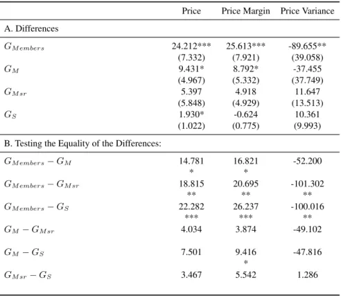
Table 2.3 presents the average outcome difference across the four groups during a collusive agreement. Panel A shows the difference in outcomes for those groups when there is an active cartel. Estimations use panel data and consider station and time fixed effects. Table 2.3 gives us a first indication that prices and margins are greater during the cartel for the stations that took part on the agreement and for those located inside the same municipalities. We also observe lower price variance among cartel members.
TABLE 2.3. Effect of a Cartel onset for Cartel Members and other Submarkets, Simple Difference
Price Price Margin Price Variance
A. Differences
GM embers 24.212*** 25.613*** -89.655**
(7.332) (7.921) (39.058)
GM 9.431* 8.792* -37.455
(4.967) (5.332) (37.749)
GM sr 5.397 4.918 11.647
(5.848) (4.929) (13.513)
GS 1.930* -0.624 10.361
(1.022) (0.775) (9.993)
B. Testing the Equality of the Differences:
GM embers−GM 14.781 16.821 -52.200
* *
GM embers−GM sr 18.815 20.695 -101.302
** ** **
GM embers−GS 22.282 26.237 -100.016
*** *** **
GM −GM sr 4.034 3.874 -49.102
GM −GS 7.501 9.416 -47.816
*
GM sr−GS 3.467 5.542 1.286
Note: Robust standard errors in parentheses *** p<0.01, ** p<0.05, * p<0.1. All currency figures are in cents of Reais deflated for September 2015. Data are from 555 municipalities in Brazil from 2001:7 - 2011:12 at the station-level on weekly basis.
Results indicate that prices and margins for cartel member stations are 24.2and25.6cents of Reais higher, respectively, and price variance is lower during cartel operation compared to all other stations. Stations operating in the same market as the collusive stations also practice price levels and margins9.4and8.8cents higher than the overall market, respectively.
not quite different from the other stations being considered. The same can be said about prices for�Sthat present a small but significant increment, according to panel A.
Table 2.3 confirms the well-known result that cartel agreements increase prices and margins and reduce price variances among its members. It also shows that the effect is not limited to the firms that take part in the cartel, but there is a spillover effect in prices and margins to stations situated in the same municipalities.
3.2 Regression Analysis:
In this subsection we perform an econometric analysis to disentangle the changes that are due to the binding cartel agreement from those that were driven by market structure changes. Also, to better approach our research question, we estimate all geographical niches together in such a way that the control group is all the other stations out of the State where the collusion was taking place, that is, all other stations in the Brazilian territory that were out of a cartel agreement. Our proposed specification is:
�it= �0+�1 ∗�(�∈�M embers)∗�+�2∗�(�∈�M)∗�+�3∗�(�∈�M sr)∗�
+�4∗�(�∈�S)∗� +��it+�i+�t+�it
(2.1)
where �it is the outcome variables (price levels, margins or price variance) for station�in week�, I(·) is an indicator function that recalls each one of the appointed groups - �M embers, �M, �M sr and �S and � = 1 if cartel is operating and zero otherwise. �i is a station fixed effect,�t is a time fixed effect set in weeks,�it is a vector of time-varying market structure as described in the previous section,�itis the error term. We compute the described model using panel data with gas station and time fixed effects.
The parameter �1 captures the effect of the cartel agreement among the stations that in
fact took part in the offense, �2 represents the effect on the stations that are part of the same
competitive market but do not partake in the collusion, the stations that are actually operating in the same municipalities, while �3 captures the effect of the cartel on stations in nearby
municipalities and finally �4 captures the effect on the other stations located elsewhere in the
same State.
that is, the cartel is dismembered. This way we know that during this period the cartel was active and we do not contaminate our control group with a potential cartelized period. We will come back to this shortly in the next subsection.
Results from the estimation of equation 2.1 are presented in table 2.4. We measure the direct effect (effect on the Members) of a cartel on prices and margins to be approximate25
cents per liter. All prices are measured in cents of local currency (Reais). Regarding the other groups of interest, for the most part we find that the cartel activity has no spillover effects on other submarkets with the exception of prices on stations located inside the same city. We do find an economical and statistical increase in prices among the stations that compete within the same market as the cartelized stations. Our estimates suggest this indirect effect of the cartel on prices to be, on average, an increase of10.15cents per liter.
TABLE 2.4. Effect of a Cartel on Price Levels, Margins and Variance
Price Level Price Margin Price Variance
(1) (2) (1) (2) (1) (2)
GM embers 25.836*** 25.340*** 24.680*** 24.733*** -113.572** -112.185**
(8.386) (8.292) (8.056) (8.038) (47.001) (46.722)
GM 10.152* 9.196* 8.320 8.468 -38.799 -37.239
(5.187) (5.215) (5.311) (5.283) (38.789) (36.679)
GM sr 3.511 3.602 3.588 3.672 15.396 12.440
(5.076) (4.559) (4.516) (4.457) (13.800) (14.653)
GS 1.657 0.306 -0.449 -0.765 11.187 14.730
(1.176) (1.022) (0.885) (0.922) (10.618) (11.323)
controls no yes no yes no yes
station FE yes yes yes yes yes yes
time FE yes yes yes yes yes yes
Constant 383.344*** 204.144*** 52.184*** 52.986*** 94.093*** 436.136***
(2.206) (13.641) (2.167) (2.495) (24.202) (71.366)
Observations 1,976,412 1,790,808 1,792,652 1,790,808 1,975,183 1,790,259
R-squared 0.766 0.797 0.118 0.120 0.046 0.068
Number of cod_id 19,452 19,312 19,312 19,312 19,446 19,307
Note: Robust standard errors in parentheses *** p<0.01, ** p<0.05, * p<0.1. All currency figures are in cents of Reais deflated for September 2015. Data are from 555 municipalities in Brazil from 2001:7 - 2011:12 at the station-level on weekly basis. The full table is presented in appendix 2.8.
The existence of this indirect effect comes as no surprise given that by competing in the same market, prices are a complementary strategy for player playing a Bertrand game: each station’s best strategy is to charge higher prices if its competitor is also charging higher prices.
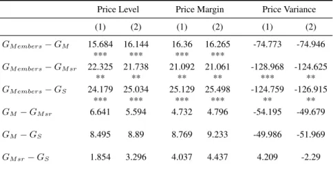
TABLE2.5. Tests of the difference in coefficients for the Effect of a Cartel
Price Level Price Margin Price Variance
(1) (2) (1) (2) (1) (2)
GM embers−GM 15.684 16.144 16.36 16.265 -74.773 -74.946
*** *** *** ***
GM embers−GM sr 22.325 21.738 21.092 21.061 -128.968 -124.625
** ** ** ** *** **
GM embers−GS 24.179 25.034 25.129 25.498 -124.759 -126.915
*** *** *** *** ** **
GM−GM sr 6.641 5.594 4.732 4.796 -54.195 -49.679
GM−GS 8.495 8.89 8.769 9.233 -49.986 -51.969
GM sr−GS 1.854 3.296 4.037 4.437 4.209 -2.29
Note: Robust standard errors in parentheses *** p<0.01, ** p<0.05, * p<0.1. All currency figures are in cents of Reais deflated for September 2015. Data are from 555 municipalities in Brazil from 2001:7 - 2011:12 at the station-level on weekly basis.
statistical spillover effect of cartel on prices, as seen on table 2.4, the effect cannot be said to be different than the non-significant effect of the other submarkets.
Broadly, we see that results from table 2.4 are very similar to table 2.3. Adding market structure and estimating all groups together have not changed our results significantly.
Overall, our results suggest that by interacting directly with firms that are under a cartel agreement, non-collusive firms also increase the magnitude of their prices as a result of direct Bertrand competition. The spillover effect of the cartel, however, is limited to firms that compete in the same market. Mutual distributors and commuters are insufficient to generate this spillover effect.
3.3 Robustness Check:
In this subsection we perform a difference-in-difference analysis considering four different periods of cartel operation15. First we consider the period described in the court documents, but
instead of discarding the observations for the period before the supposed onset of the cartel (as we did in the previous subsection), we consider it as off cartel period. This way we can perform the double difference estimation. Following, we test for three additional windows allowing for the cartels to have started before the date the authorities began their investigation.
Table 2.6 report our estimated results using panel data with gas station and week fixed effects. We observe from panel A that for all cartel operation windows, prices are higher for cartel members and stations located in the same municipalities, the magnitude, however, is
15All previous exercises disregarded the period before and after the cartel. The period before because we argued it
could be contaminated by active cartel operation; the period after because stations suffered an antitrust enforcement and could be behaving accordingly.
about half what we estimated on table 2.4. Panel B and C display the results for price margins and variance, respectively. As seen in table 2.4, margins are still significantly higher for cartel members but not other operating stations. However, the same can not be said about price variance that are no longer significantly smaller for cartel member.
When we compare and test the difference of the estimated coefficients on table 2.7 we find the coefficients for prices and margins on cartel members to be statistically different than stations in the same municipality and elsewhere in the State, but not when contrasted to stations in nearby municipalities. The effect seems the same among all other stations analyzed except for prices for stations inside the same municipality that are consistently higher than for stations elsewhere in the State.
Despite some differences concerning the stations inside the mesoregion, the results emerging from the robustness exercises tend to confirm our main result that the effect of a cartel agreement is strongly restricted to stations that took part in the offense and have a small but significant effect on prices among stations operating in the same municipality. That is, the cartel has a spillover effect limited to increasing prices in station competing inside the same relevant market.
4 Conclusion
In this paper, we intended to test the existence of cartel spillover effect, and if existent, how far does it spread out. Our objective in this paper was to quantify the impact of cartel agreements on pricing patterns not only within the members of the collusive agreement but also among players outside of it by investigating price behavior on related markets.
We investigated if the existence of an operating cartel in a market has any effect on price levels, price margins and price variance in other nearby and related retail gasoline stations. We believe our dataset is particularly apt to study this research question because we have multiple cases of price fixing cartels in the retail gasoline market in Brazil for which we have extensive information based on court documents and the national petroleum agency’s data. In addition, the separation of ownership in Brazil between gasoline producers and retailers allows us to separate and measure the spillover effect more accurately than in markets where production and retailing of gasoline are owned by the same players.
TABLE2.6. Robustness Check: Effect of a Cartel on Price Levels, Margins and Variance
Court docs date 4 weeks prior 13 weeks prior 26 weeks prior
A: Price Level
GM embers 13.907** 13.859** 13.775** 13.394**
(6.349) (6.302) (6.252) (6.278)
GM 3.397** 3.198** 3.161** 2.880*
(1.501) (1.469) (1.446) (1.472)
GM sr 4.425 4.210 3.825 3.040
(3.024) (3.129) (3.385) (3.713)
GS -0.511 -0.554 -0.590 -0.390
(1.027) (1.023) (1.045) (1.056)
controls yes yes yes yes
station FE yes yes yes yes
time FE yes yes yes yes
Constant 206.542*** 206.520*** 206.496*** 206.396***
(11.671) (11.672) (11.672) (11.675)
Observations 2,298,131 2,298,190 2,298,190 2,298,190
R-squared 0.787 0.787 0.787 0.787
Number of cod_id 20,621 20,621 20,621 20,621
B: Price Margins
GM embers 11.418* 11.360* 11.248* 10.836*
(6.562) (6.515) (6.469) (6.498)
GM 0.793 0.614 0.555 0.275
(1.669) (1.610) (1.570) (1.618)
GM sr 3.411 3.152 2.723 1.842
(2.807) (2.902) (3.108) (3.353)
GS -0.831 -0.912 -1.033 -1.008
(1.001) (0.991) (1.009) (1.029)
controls yes yes yes yes
station FE yes yes yes yes
time FE yes yes yes yes
Constant 50.978*** 51.018*** 51.050*** 51.121***
(1.720) (1.723) (1.719) (1.717)
Observations 2,298,131 2,298,190 2,298,190 2,298,190
R-squared 0.123 0.123 0.123 0.123
Number of cod_id 20,621 20,621 20,621 20,621
C: Price Variance
GM embers -12.164 -12.534 -11.838 -11.731
(23.416) (23.105) (23.004) (22.923)
GM 5.205 6.894 8.355 8.826
(12.978) (12.964) (12.760) (12.702)
GM sr -31.664** -31.965*** -30.606** -30.828**
(12.256) (12.084) (12.350) (12.271)
GS -4.523 -3.579 -1.799 -1.435
(7.946) (7.948) (7.796) (7.869)
controls yes yes yes yes
station FE yes yes yes yes
time FE yes yes yes yes
Constant 497.272 325.672 344.870 334.518
(.) (.) (.) (.)
Observations 2,297,415 2,297,474 2,297,474 2,297,474
R-squared 0.065 0.065 0.065 0.065
Number of cod_id 20,616 20,616 20,616 20,616
Note: Robust standard errors in parentheses *** p<0.01, ** p<0.05, * p<0.1. All currency figures are in cents of Reais deflated for September 2015. Data are from 555 municipalities in Brazil from 2001:7 - 2011:12 at the station-level on weekly basis.
TABLE 2.7. Robustness Check: Tests of the difference in coefficients for the Effect of a Cartel
Court docs date 4 weeks prior 13 weeks prior 26 weeks prior
Price Level
GM embers−GM 10.51 10.661 10.614 10.514
** ** ** **
GM embers−GM sr 9.482 9.649 9.95 10.354
GM embers−GS 14.418 14.413 14.365 13.784
** ** ** **
GM−GM sr -1.028 -1.012 -0.664 -0.16
GM−GS 3.908 3.752 3.751 3.27
** ** ** **
GM sr−GS 4.936 4.764 4.415 3.43
Price Margins
GM embers−GM 10.625 10.746 10.693 10.561
* ** ** *
GM embers−GM sr 8.007 8.208 8.525 8.994
GM embers−GS 12.249 12.272 12.281 11.844
* * * *
GM−GM sr -2.618 -2.538 -2.168 -1.567
GM−GS 1.624 1.526 1.588 1.283
GM sr−GS 4.242 4.064 3.756 2.85
Price Variance
GM embers−GM -17.369 -19.428 -20.193 -20.557
GM embers−GM sr 19.5 19.431 18.768 19.097
GM embers−GS -7.641 -8.955 -10.039 -10.296
GM−GM sr 36.869 38.859 38.961 39.654
** ** ** **
GM−GS 9.728 10.473 10.154 10.261
GM sr−GS -27.141 -28.386 -28.807 -29.393
** ** ** **
Note: Robust standard errors in parentheses *** p<0.01, ** p<0.05, * p<0.1. All currency figures are in cents of Reais deflated for September 2015. Data are from 555 municipalities in Brazil from 2001:7 - 2011:12 at the station-level on weekly basis.
the cartel, however, is limited to firms that compete in the same market. Mutual distributors and commuters are insufficient to generate any spillover effect of the cartel. Our results also corroborate the common definition of the municipality as the relevant market in the retail gasoline market.
In terms of magnitudes, a cartel increases prices among members, on average, 26cents of
national average. No spillover effect is observed on margins or price variance, or in stations in other related markets.
5 Appendix
FIGURE 2.2. Evolution of prices and costs for Cartelized stations
(a) Manaus (b) Teresina
(c) Recife (d) Joao Pessoa
(e) Natal (f) Goiania
Continued from previous page
(g) Cuiaba (h) Varzea Grande
(i) Belo Horizonte (j) Vitoria
(k) Bauru (l) Londrina
(m) Santa Maria (n) Caxias do Sul
TABLE2.8. Effect of a Cartel on Price Levels, Margins and Variance (complete)
Price Level Price Margin Price Variance
(1) (2) (1) (2) (1) (2)
GM embers 25.836*** 25.340*** -113.572** -112.185** 24.680*** 24.733***
(8.386) (8.292) (47.001) (46.722) (8.056) (8.038)
GM 10.152* 9.196* -38.799 -37.239 8.320 8.468
(5.187) (5.215) (38.789) (36.679) (5.311) (5.283)
GM sr 3.511 3.602 15.396 12.440 3.588 3.672
(5.076) (4.559) (13.800) (14.653) (4.516) (4.457)
GS 1.657 0.306 11.187 14.730 -0.449 -0.765
(1.176) (1.022) (10.618) (11.323) (0.885) (0.922)
Cost Proxy 0.539*** -1.079***
(0.040) (0.188)
Nostations in the market -0.053** 0.165 -0.058**
(0.021) (0.122) (0.024)
Nodiff brands in the market 0.082 2.352 0.073
(0.228) (1.496) (0.207)
Nostations branded in the market 0.039 -0.307 0.067**
(0.024) (0.226) (0.027)
Proportion of low brands and independents -0.436 2.745 0.016
(0.403) (2.838) (0.329)
Density of stations per municipality 3.141 12.925 -6.829
(10.858) (58.721) (8.345)
Branded (dummy) 0.075 1.872 -0.642
(0.547) (3.162) (0.487)
Ale brand 1.051 0.162 0.441
(0.869) (4.872) (0.844)
BP brand -2.848 -11.133 -4.662
(3.341) (12.147) (3.151)
BR brand -0.005 -2.326 0.050
(0.733) (3.512) (0.682)
Ipiranga brand 0.678 -4.150 0.435
(0.597) (3.549) (0.568)
Chevron brand 0.654 -9.256 0.629
(0.849) (6.098) (0.800)
Cosan brand 1.538 4.272 0.817
(0.957) (5.899) (0.935)
Esso brand -1.579*** 3.891 -1.686***
(0.552) (3.195) (0.548)
Repsol brand -0.582 1.749 -1.308
(1.120) (11.364) (1.087)
Shell brand 1.277 -4.636 1.004
(1.422) (7.523) (1.278)
Texaco brand 0.579 0.764 0.558
(0.713) (4.450) (0.692)
Total brand 0.656 -7.324 1.278
(1.396) (4.947) (1.319)
station FE yes yes yes yes yes yes
time FE yes yes yes yes yes yes
Constant 383.344*** 204.144*** 94.093*** 436.136*** 52.184*** 52.986***
(2.206) (13.641) (24.202) (71.366) (2.167) (2.495)
Observations 1,976,412 1,790,808 1,975,183 1,790,259 1,792,652 1,790,808
R-squared 0.766 0.797 0.046 0.068 0.118 0.120
Number of cod_id 19,452 19,312 19,446 19,307 19,312 19,312
.
Note: Robust standard errors in parentheses *** p<0.01, ** p<0.05, * p<0.1. All currency figures are in cents of Reais deflated for September 2015. Data are from 555 municipalities in Brazil from 2001:7 - 2011:12 at the station-level on weekly basis.
TABLE2.9. Robustness Check: Effect of a Cartel on Price Levels, Margins and Variance (complete)
Court docs date 4 weeks prior 13 weeks prior 26 weeks prior
A: Price Level
GM embers 13.907** 13.859** 13.775** 13.394**
(6.349) (6.302) (6.252) (6.278)
GM 3.397** 3.198** 3.161** 2.880*
(1.501) (1.469) (1.446) (1.472)
GM sr 4.425 4.210 3.825 3.040
(3.024) (3.129) (3.385) (3.713)
GS -0.511 -0.554 -0.590 -0.390
(1.027) (1.023) (1.045) (1.056)
Cost Proxy 0.521*** 0.521*** 0.521*** 0.522***
(0.035) (0.035) (0.035) (0.035)
Nostations in the market -0.031 -0.032 -0.032 -0.032
(0.024) (0.024) (0.023) (0.023)
Nodiff brands in the market 0.177 0.177 0.180 0.178
(0.207) (0.206) (0.205) (0.205)
Nostations branded in the market 0.014 0.015 0.015 0.015
(0.027) (0.027) (0.027) (0.027)
Proportion of low brands and independents -0.388 -0.390 -0.397 -0.397
(0.409) (0.410) (0.413) (0.414)
Density of stations per municipality 3.599 3.456 3.443 3.189
(6.851) (6.861) (6.868) (6.890)
Branded (dummy) -0.066 -0.067 -0.060 -0.058
(0.426) (0.426) (0.426) (0.427)
Ale brand 1.407** 1.407** 1.403** 1.392**
(0.589) (0.589) (0.589) (0.589)
BP brand -0.880 -0.879 -0.892 -0.901
(3.044) (3.045) (3.048) (3.050)
BR brand 0.088 0.093 0.097 0.098
(0.580) (0.580) (0.580) (0.581)
Ipiranga brand 0.918* 0.925* 0.932* 0.939*
(0.500) (0.499) (0.498) (0.498)
Chevron brand 0.473 0.482 0.486 0.496
(0.787) (0.786) (0.785) (0.785)
Cosan brand 1.957** 1.961** 1.954** 1.944**
(0.913) (0.913) (0.915) (0.916)
Esso brand -1.272** -1.269** -1.271** -1.269**
(0.532) (0.532) (0.533) (0.532)
Repsol brand 0.164 0.160 0.152 0.153
(1.038) (1.037) (1.037) (1.037)
Shell brand 0.967 0.968 0.969 0.974
(1.186) (1.186) (1.185) (1.185)
Texaco brand 0.592 0.596 0.599 0.604
(0.627) (0.626) (0.625) (0.624)
Total brand 0.793 0.830 0.841 0.795
(1.279) (1.276) (1.275) (1.289)
station FE yes yes yes yes
time FE yes yes yes yes
Constant 206.542*** 206.520*** 206.496*** 206.396***
(11.671) (11.672) (11.672) (11.675)
Observations 2,298,131 2,298,190 2,298,190 2,298,190
R-squared 0.787 0.787 0.787 0.787
Number of cod_id 20,621 20,621 20,621 20,621
.
Note: Robust standard errors in parentheses *** p<0.01, ** p<0.05, * p<0.1. All currency figures are in cents of Reais deflated for September 2015. Data are from 555 municipalities in Brazil from 2001:7 - 2011:12 at the station-level on weekly basis.
Continued from previous page
Court docs date 4 weeks prior 13 weeks prior 26 weeks prior
B: Price Margin
GM embers 11.418* 11.360* 11.248* 10.836*
(6.562) (6.515) (6.469) (6.498)
GM 0.793 0.614 0.555 0.275
(1.669) (1.610) (1.570) (1.618)
GM sr 3.411 3.152 2.723 1.842
(2.807) (2.902) (3.108) (3.353)
GS -0.831 -0.912 -1.033 -1.008
(1.001) (0.991) (1.009) (1.029)
Nostations in the market -0.042 -0.042 -0.042 -0.042
(0.030) (0.030) (0.030) (0.030)
Nodiff brands in the market 0.166 0.165 0.166 0.162
(0.180) (0.179) (0.179) (0.178)
Nostations branded in the market 0.040 0.040 0.041 0.042
(0.035) (0.035) (0.035) (0.035)
Proportion of low brands and independents 0.122 0.120 0.115 0.114
(0.376) (0.376) (0.375) (0.376)
Density of stations per municipality -1.807 -1.950 -2.011 -2.288
(5.325) (5.320) (5.324) (5.329)
Branded (dummy) -0.781** -0.781** -0.777* -0.777*
(0.396) (0.396) (0.396) (0.396)
Ale brand 0.948 0.946 0.938 0.922
(0.604) (0.604) (0.604) (0.603)
BP brand -0.692 -0.686 -0.688 -0.692
(3.836) (3.834) (3.827) (3.823)
BR brand 0.251 0.257 0.260 0.262
(0.551) (0.552) (0.552) (0.552)
Ipiranga brand 0.622 0.629 0.634 0.637
(0.491) (0.490) (0.490) (0.490)
Chevron brand 0.341 0.348 0.352 0.360
(0.751) (0.750) (0.750) (0.749)
Cosan brand 0.911 0.916 0.911 0.905
(0.920) (0.920) (0.920) (0.921)
Esso brand -1.522*** -1.517*** -1.517*** -1.512***
(0.541) (0.541) (0.542) (0.542)
Repsol brand -0.217 -0.221 -0.231 -0.241
(1.031) (1.030) (1.029) (1.030)
Shell brand 0.671 0.670 0.668 0.668
(1.067) (1.066) (1.066) (1.065)
Texaco brand 0.525 0.531 0.536 0.543
(0.625) (0.625) (0.624) (0.623)
Total brand 1.164 1.196 1.207 1.189
(1.325) (1.321) (1.320) (1.325)
station FE yes yes yes yes
time FE yes yes yes yes
Constant 50.978*** 51.018*** 51.050*** 51.121***
(1.720) (1.723) (1.719) (1.717)
Observations 2,298,131 2,298,190 2,298,190 2,298,190
R-squared 0.123 0.123 0.123 0.123
Number of cod_id 20,621 20,621 20,621 20,621
.