ESCOLA DE PÓS-GRADUAÇÃO EM ECONOMIA
–
EPGE
FUNDAÇÃO GETÚLIO VARGAS
JOÃO BARATA RIBEIRO BLANCO BARROSO
ESSAYS ON INTERNATIONAL PRICES AND THE
SUBJACENT MARKET STRUCTURE
JOÃO BARATA RIBEIRO BLANCO BARROSO
ESSAYS ON INTERNATIONAL PRICES AND THE
SUBJACENT MARKET STRUCTURE
Tese submetida à Escola de Pós-Graduação em Economia
da Fundação Getulio Vargas como requisito de obtenção do
título de Doutor em Economia
Orientador: Renato Galvão Flôres Junior
Agradeço,
Aos meus pais, pelo amor e apoio incondicional
Ao meu orientador, Renato Flôres, por acreditar e guiar este projeto a uma boa conclusão Aos colegas da Divisão do Balanço de Pagamentos do Banco Central Do Brasil, pela amizade, encorajamento e auxílio técnico inestimável
Resumo
Resumo. Esta tese utiliza a informação contida em preços internacionais para identificar parâmetros de modelos de comércio sob competição imperfeita, desta forma permitindo inferência sobre o comportamento das exportações, sobre os ganhos de troca da abertura comercial e sobre a variedade de bens produzidos domesticamente. Em primeiro lugar, investigamos o repasse cambial, no longo prazo, para os preços praticados por exportadores brasileiros. O foco no longo prazo permite controlar os efeitos da rigidez de preço no curto prazo, de maneira que o repasse incompleto evidencie competição imperfeita com preços flexíveis. Em segundo lugar, calculamos os ganhos de troca de novas variedades de bens importados baseando-nos em estimativas para as elasticidades de substituição desagregadas. Finalmente, qualificamos a ênfase da literatura de comércio em ganhos de eficiência no lugar de ganhos de variedade, demonstrando que a variedade de bens produzidos domesticamente se amplia após aberturas comerciais desde que as firmas tenham uma margem de decisão em bens intermediários ou na qualificação da mão de obra. Palavras-Chave: comércio internacional, competição imperfeita, preços internacionais, repasse cambial, ganhos de troca, variedade de bens
Abstract. The thesis uses international price data to identify parameters of trade models with imperfect competition, therefore allowing inference on exchange rate behavior, gains from trade and variety of domestic goods. First, we investigate Brazilian exporters pricing behavior over the long-run following destination specific exchange rate shocks. We find evidence of incomplete exchange-rate pass-through in the long-run, which supports the market structure explanations over short-run sticky-price explanations. Second, we calculate import price indexes and the implied welfare gains from new varieties of imported goods, based on disaggregated estimates of elasticity of substitution parameters. Finally, we qualify standard results in the literature that point to a reduction in domestic varieties after trade liberalization; domestic varieties may expand if we introduce
an additional margin in firms‟ technology, such as intermediate goods or high skilled labor.
Contents
Introduction
1
Chapter 1. Pricing-to-market by Brazilian
Exporters: a Panel Cointegration Approach
2
Chapter 2. Gains from Imported
Varieties in the Brazilian Economy
26
Chapter 3. Domestic Varieties Under
Free Trade: Shrinking or Expanding?
1
Introduction
This thesis is composed of three essays with a common interest on trade under imperfect competition. From a technical standpoint, we use different strategies to identify primitive parameters from information on international prices. From an applied standpo int, the primitive parameters underlying price behavior have wide-range implications; from the conduct of exchange-rate policy to the welfare consequences of trade; from aggregation biases in trade elasticities to the skill-premium consequences of foreign competition.
The first chapter investigates Brazilian exporters pricing behavior over the long-run following destination specific exchange rate shocks. The panel cointegration method of Bai, Kao and Ng (2009) is shown to identify the long-run parameter of interest. We find evidence of incomplete exchange-rate pass-through in the long-run, which supports the market structure explanations of Krugman (1986) over short-run sticky-price explanations. Optimal incomplete pass-through implies lower risk premium from short-run sticky-prices; therefore, it changes incentives for exchange rate policy.
The second chapter estimates import price indexes and the implied welfare gains from new varieties of imported goods. A lot of care is taken with heterogeneity in consumers‟ taste parameters over different kinds of goods, as well as heterogeneity in
firms‟ technology parameters over different intermediate goods. To identify this wealth of
elasticities of substitution parameters, we assembled import price data for a large array of goods and explored heteroscedasticity in the panel dimension of each of these data sets. Elasticities of substitution are shown to have systematic relations to market structure indicators. They also point to aggregation bias in standard estimates of aggregate elasticities of substitution and aggregate price-indexes.
2
Pricing-to-market by Brazilian
Exporters: a Panel Cointegration Approach
Abstract
This paper investigates Brazilian exporters pricing behavior over the long-run following destination specific exchange rate shocks. The panel cointegration method of Bai, Kao and Ng (2009) is shown to identify the long-run parameter of interest. The method crucially depends on identification and controlling for the common trend in prices to different countries, a trend which is structurally interpreted, like originally proposed by Kneeter (1989), as the exporter‟s marginal cost. We find evidence of incomplete exchange-rate pass-through in the long-run, which supports the market structure explanations of Krugman (1986), known in the literature as pricing-to-market, over contending short-run sticky-price explanations. The degree of long-run pass-through is also shown to be positively related to technological intensity in the sector, a proxy for low elasticity of substitution of varieties.
JEL Classification: C52, D43, F12, F14,F31, L13
3 1. Introduction
With sufficiently segmented international markets, exporters may set country specific prices to reflect local demand and competition conditions, a behavior Krugman (1986) called pricing-to-market. The concept is relevant for many empirical puzzles in international economics, such as incomplete exchange rate pass-through to exporter prices and persistent deviations from purchasing power parity. The main advantage over contending explanations, the leading one being sticky prices set by exporters in local currencies, is the optimal character of the pricing rules1 and the possible accounting for persistent shocks on relative international prices2. This paper follows the empirical tradition of identifying microeconomic pricing-to-market behavior by resort to exporter‟s destination specific mark-up adjustments after exchange rate shocks [Krugman (1986), Kneeter (1989)]. Advancing previous methods, we look for credible estimates of long run pricing-to-market effects on Brazilian exports. By definition, the effect cannot be attributed to sticky price and other short run explanations of incomplete exchange-rate pass-through. On the contrary, it amounts to strong evidence in favor of market structure explanations, the more so considering it refers to exporters from a developing country where it is least expected. Additionally, we look for patterns of behavior across different industries, a significant undertaking in face of the large number of imperfect competition models that may explain the results.
Krugman‟s (1986) original strategy to identify pricing-to-market behavior was trying to control for exogenous trends in prices common across all export destinations in order to recognize divergent trends after a large real exchange rate shock; this was implemented for German export data. Kneeter (1989) developed this basic insight further. The author proposed a panel framework that controls for common trends in prices by the inclusion of a time effect. He also provided structural interpretation for the common trend as the production cost of the marginal unit, such as can be deduced from the optimization
1
Sticky local currency prices have welfare implications under flexible exchange rate regimes through the addition of a risk premium term to import and export prices [Sutherland (2005)]; by reducing optimal variability, pricing-to-market have a direct bearing on risk premium and welfare.
2
4 problem of a representative firm exporting to many destinations. The model proposed in this paper has very similar interpretation; so, it is worth getting at some details of Kneeter‟s econometric specification. The author singles out the bilateral exchange rate, measured as
the price of exporter currency in each destination country‟s currency, as the relevant country specific shock, from which to gauge the presence and quantitative magnitude of pricing-to-market behavior. Measuring prices in the exporter‟s currency, the degree of pricing-to-market can be assessed by the partial effect of the bilateral exchange rate on export price while holding marginal cost fixed. Expressing the variables in logarithms, this coefficient measures the effect of the exchange rate on exporter‟s mark-up over marginal costs. Also, since foreign prices are just the sum of the exporter price and the exchange rate, one plus the coefficient measures the exchange rate pass-through to foreign consumers due to mark-up adjustments.
An important result from Kneeter (1989) is that U.S. exporters in most industries appear to fully or over pass-through exchange rate movements to foreign consumers. As noted by the author, instead of the usual assumption of foreign demand curve becoming more elastic as price rises, such coefficients would require just the opposite assumption (for mark-ups are inversely related to the elasticity of demand). This sort of result persisted throughout the literature: there is wide dispersion, usually around full pass-through levels and many coefficients have significant but counterintuitive signs. For a recent example, Méjan (2004) found exactly those results for massive data sets on Germany, United States, France, Italy, Japan and United Kingdom exporters, with volume and price data organized in much disaggregated sectors. On a more optimistic tone, Méjan interpreted the wide dispersion as room for structural, microeconomic explanations. In the most recently published paper on the subject, Bugamelli and Tedeschi (2008) report the same pattern of result after many variations of Kneeter‟s basic specification. Because their estimated coefficients bundle many different products, the dispersion is not as accentuated as in
5 attempts at dynamic panel models with quarterly or monthly data, such as Takagi and Yoshida (2001), on Japanese exports. But the inclusion of lagged price as an explanatory variable, with the associated dynamic panel methodology, leads to the same pattern of results.
The main contribution from this paper is to extend Kneeter‟s panel method to allow for long-run relations between the variables and to actually estimate the long-run parameters. We trusts long run relations will provide a clearer picture on pricing-to-market behavior, with coefficients less dispersed, more plausibly signed and easier to connect with microeconomic fundamentals. In addition, because nominal rigidities have no place in the long-run, the estimated coefficients may discriminate between market structure and sticky prices explanations of incomplete pass-through. At a conceptual level, an important advance is to model the common marginal cost trend as a stochastic process on par with the price and exchange rate processes, with the explicit possibility of equilibrium relations among all of the variables. Long-run relations are modeled as cointegration among integrated processes, which is a restricted but useful interpretation. For example, this rules out mean reverting residuals with long memory, as well as overlooks possible inference problems from near unit root series. In a sense, though, the econometric method proposed in this paper is genuinely more general then previous methods used in the literature, since estimates are consistent even if some of the variables are stationary in levels as previous authors have maintained. The unit-root hypothesis is necessary only for a long-run interpretation of the coefficients; even so, the paper tests this null against stationarity with panel techniques that have greater power then single series tests.
The appropriate econometric theory to address long-run issues in a panel framework was only recently developed. Philips and Moon (1996) were the first to propose consistent estimators for panel cointegration vectors with the concomitant development of the asymptotic theory for sequential and simultaneous limits in the two panel dimensions. An important shortcoming was the assumption of independent errors along the cross-section dimension. To overcome this difficulty, Bai, Kao and Ng (2009) developed a “second
6 appropriate estimator. Indeed, the behavioral model proposed in this paper has an exact mapping to Bai, Kao and Ng econometric specification. Nevertheless, it should be stressed that, while the common factors are just an econometric device in their model, here we adopt the much stronger structural interpretation of a common marginal cost trend in export prices to different destinations3. As already mentioned, the estimator does not require pre-testing the variables for unit-root against the stationarity alternative. However, in order to check if our initial concerns were of any consequence, we also applied Bai and Kao (2002) panel unit root test to the bilateral exchange rate and export price series.
Another contribution from the paper is the use of product classification to uncover possible microeconomic patterns in the estimated pass-through coefficients. Although the approach is similar to Bugamelli and Tedeschi (2008), two important differences have a bearing on the results. First, the authors used unit values throughout, estimating the common effect for a group of products by including an associated dummy variable. In contrast, this paper bundles the products from the start and calculates price indexes on which the whole analysis is conducted. Second, the actual classification scheme is different; the one used here is closely based on technological intensity. As a research principle, the discipline of building the indexes before obtaining the estimates lends more credibility to any pattern eventually found, since one minimizes snooping through many different aggregations. It also potentially ameliorates the measurement error from using unit values as proxies for prices, under the assumption of independent errors. As for the classification system, we have used it in parallel research which actually suggests some connections with structural preference and market structure parameters.
The remainder of the paper is organized as follows. Section 2 describes the data and limitations. Section 3 reports results on panel unit-root tests relevant for interpreting the results. Section 4 is the heart of the paper, explaining the structural model, the econometric model and the estimation results. Section 5 discusses the panel cointegration results in relation to previous estimates and looks for microeconomic patterns. Section 6 concludes.
3
7 2. Data description and limitations
The data sample ranges from the first quarter of 1997 to the third quarter of 2006, which amounts to 39 periods. Depending on the sector, the number of export destination countries can be as little as 29 and as much as 53. On the one hand, the small sample size in the two panel dimensions, time and country, could raise problems for the asymptotic inferences. On the other hand, the estimator used here was shown to have good finite sample properties in simulation experiments reported by Bai, Kao and Ng (2006). Indeed, the mean bias and standard deviation of the estimates keep their good asymptotic properties in samples as small as 20 in both panel dimensions. More importantly, the estimator has much better properties in small samples than the alternatives4.
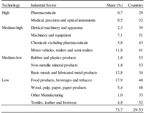
As shown in Table 1, Brazilian exports of manufactures were classified in thirteen sectors according to technological intensity. There are many reasons to adopt some level of aggregation. First, this reduces data to manageable proportions. Second, price indexes average out measurement error in the price data. Third, it permits to investigate a possible relationship between pass-through and technological intensity, throwing some light on the microeconomic structure driving the results. Finally, Brazilian official institutions often use this classification scheme, which was developed by OCDE in 1995 (Classification of High-technology Products and Industries), thus facilitating research communication. Some sectors from the original classification, namely aviation, ship building and oil, have been excluded due to insufficient number of export destination countries. The sector share in the table refers to the value exported in the third quarter of 2006 relative to total manufacturing export.
Table 1 also reports the number of countries in each sector. The criteria for including a country in a particular sector were positive export to this country in all periods and for a significant fraction of the products from the sector. The selection rule ensures a balanced panel in each sector, as well as high quality export price indexes. The rule could lead to selection bias. However, the most likely reason for low trade volume is trade barrier,
4
8 and the pricing behavior exporters would have in case of no barrier should be independent of the actual level of the barrier. Additionally, excluded countries get none or just a small share of Brazilian exports, and it seems justified to give much less weight to these countries in the estimation of the pooled coefficient. The last section of the paper discusses the selection issue further.
Export price indexes were calculated with unit values at the finest level of the Harmonized System, an international standard for commodity classification. The Fisher index formula was used after a preliminary trimming of too extreme variation, very unlikely to reflect price developments. For each country, in each sector, an export price series was constructed. Unit values are poor measures of price. Still, they are readily available and very much used in empirical studies on international prices. The inclusion of country specific effects should capture any measurement error that survives aggregation. As already mentioned, one reason to use aggregate price indexes is to average out the likely measurement errors in prices. On the other hand, the more aggregated sector classification we use, the less reasonable our structural interpretation of the data. Relative to other studies with a similar panel approach, our choice in this trade-off involves more aggregation.
Table 1. Industrial sectors by technological intensity: share and number of countries
Technology Industrial Sector Share (%) Countries
High Pharmaceuticals 0,7 29
Medical, precision and optical instruments 0,5 32
Medium-high Eletrical machinery and apparatus 2,3 39
Machinery and equipment 7,1 51
Chemicals excluding pharmaceuticals 5,8 43
Motor vehicles, trailers and semi-trailers 11,8 41
Medium-low Rubber and plastics products 1,8 53
Non-metallic mineral products 1,8 53
Basic metals and fabricated metal products 12,8 34
Low Food products, beverages and tobacco 17,9 46
Wood, pulp, paper, paper products 5,4 48
Other Manufacturing 1,0 33
Textiles, leather and footwear 4,8 52
9 Figure 1. Export price indexes by industrial sector; high and medium high technology Median in bold-line; other quartiles in dashed-lines; 1997:I = 100; Monetary Unit = R$
High Technology Medium-high Technology 50 100 150 200 250 I 97 III I 98 III I 99 III I 00 III I 01 III I 02 III I 03 III I 04 III I 05 III I 06 III Pharmaceuticals 50 100 150 200 I 97 III I 98 III I 99 III I 00 III I 01 III I 02 III I 03 III I 04 III I 05 III I 06 III Medical, precision and optical instruments
50 100 150 200 250 I 97 III I 98 III I 99 III I 00 III I 01 III I 02 III I 03 III I 04 III I 05 III I 06 III Eletrical machinery and apparatus
50 100 150 200 250 I 97 III I 98 III I 99 III I 00 III I 01 III I 02 III I 03 III I 04 III I 05 III I 06 III Machinery and equipment
50 100 150 200 250 300 I 97 III I 98 III I 99 III I 00 III I 01 III I 02 III I 03 III I 04 III I 05 III I 06 III Chemicals excluding pharmaceuticals
10 Figure 2. Export price indexes by industrial sector; medium-low and low technology Median in bold-line; other quartiles in dashed-lines; 1997:I = 100; Monetary Unit = R$
Medium-low Technology Low Technology 50 100 150 200 250 I 97 III I 98 III I 99 III I 00 III I 01 III I 02 III I 03 III I 04 III I 05 III I 06 III Rubber and plastics products
50 100 150 200 250 I 97 III I 98 III I 99 III I 00 III I 01 III I 02 III I 03 III I 04 III I 05 III I 06 III Non-metallic mineral products
50 100 150 200 250 300 I 97 III I 98 III I 99 III I 00 III I 01 III I 02 III I 03 III I 04 III I 05 III I 06 III Basic metals and fabricated metal products
50 100 150 200 250 I 97 III I 98 III I 99 III I 00 III I 01 III I 02 III I 03 III I 04 III I 05 III I 06 III Food products, beverages and tobacco
50 100 150 200 250 300 I 97 III I 98 III I 99 III I 00 III I 01 III I 02 III I 03 III I 04 III I 05 III I 06 III Wood, pulp, paper, paper products
11 Figure 3. Real bilateral exchange rate
Median in bold-line; other quartiles in dashed-lines; 1997:I = 100
Figure 1 and 2 summarize the export price data for each sector. The median is a rough estimate of a common trend component, while the other quartiles capture how closely country data follow this trend. As can be seen by the widening distance of the quartile-band in most sectors, the common trend appears to have a weak influence in the price data. This will be more formally studied in the next section.
Bilateral exchange rate series were corrected for consumer price inflation in each export destination country. Both the nominal exchange rate and consumer price data were obtained from the International Financial Statistics (IFS) database. After the correction, we
obtain a „real‟ exchange rate measure, from the point of view of consumers in each export
destination country. Indeed, we will often refer to the corrected exchange rate as the bilateral real exchange rate. One could argue that sector specific price inflation in each foreign country should be used in place of consumer price inflation, but this kind of data is not easily obtainable. Figure 3 summarizes exchange rate data. Compared to the price series, the common trend captured by the median seems to be much more important for exchange rates, with all the country series following it very closely.
0 20 40 60 80 100 120
I 1997
III I 1998
III I 1999
III I 2000
III I 2001
III I 2002
III I 2003
III I 2004
III I 2005
III I 2006
12 3. Results on panel unit-root
Before estimating the parameter of interest for each industry, we test all the series for unit-root using a panel technique developed by Bai and Kao (2004). The procedure is different from the usual time-series ones in at least two respects; first, it can spot low frequency movements that would otherwise go undetected, as long as they are shared by the series in the panel; second, it can pool the unit-root tests, making it harder to incorrectly accept the unit-root null for a group of time-series. The first feature, which is unique to Bai and Kao approach, will be particularly important for correctly classifying the export price index series. It is important to highlight that none of this pre-testing is necessary for the estimation of the pricing-to-market coefficient; the estimator used in the next section would be consistent even if some of the series were stationary (but it would converge more slowly). Still, pre-testing is crucial for interpreting correctly the estimated parameters.
The test decomposes each series from a panel into a common factor and an idiosyncratic component. The estimation procedure makes no assumption about integration order of the components, thus allowing testing each component separately. Common factors serve as an econometric device to capture cross-section dependence, thus overcoming the most serious deficiency of first-generation panel tests for unit-root. In contrast to the model in the next section where the structural dependency between variables is explicitly addressed, in this section we model each variable in separation from the other.
Formally, each time-series from a given panel of series is decomposed as:
yit = dit + i‟Ft + it (1)
13 For the export price series, each sector was treated as a separate panel data set, and each of these panels was modeled as in equation (1), with i indexing the export destination country. This is a reasonable setup given that the common factors influencing the price to each destination country is most likely sector specific; we have just imposed this by assumption. Admitting at most three factors, a single factor was selected in all panels.
For the exchange rate data, the common factors are mostly associated with macroeconomic conditions unrelated to the sectors. Thus, all the export destination countries were pooled in a single panel, as in equation (1), with i indexing the country. Again, admitting at most three factors, a single factor was selected for the exchange rate.
Since there are many panels, each with several time-series, we report only summary information on the testing results. Qualitative results are not sensitive to the specification of the deterministic component; but we report results under different assumptions.
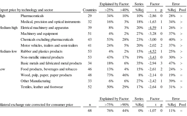
Table 2. PANIC test for unit root; one factor; constant and time trend included 39 time periods
Series
Export price by technology and sector Countries >25% >40% %Rej t p %Rej Pool
High Pharmaceuticals 29 34% 10% 10% -2,86 0 28% >
Medical, precision and optical instruments 32 16% 3% 18% -1,63 1 34% > Medium-high Eletrical machinery and apparatus 39 8% 3% 20% -4,59 1 26% >
Machinery and equipment 51 4% 2% 27% -3,28 0 37% >
Chemicals excluding pharmaceuticals 43 53% 28% 23% -3,00 0 40% >
Motor vehicles, trailers and semi-trailers 41 24% 5% 20% -2,02 2 37% >
Medium-low Rubber and plastics products 53 4% 2% 15% -4,52 1 25% >
Non-metallic mineral products 53 43% 17% 19% -3,43 0 30% >
Basic metals and fabricated metal products 34 18% 6% 35% -2,94 3 47% >
Low Food products, beverages and tobacco 46 13% 4% 15% -2,61 2 24% >
Wood, pulp, paper, paper products 48 73% 46% 8% -2,14 0 19% =
Other Manufacturing 33 6% 6% 27% -2,42 1 39% =
Textiles, leather and footwear 52 50% 29% 17% -2,64 0 31% >
Series
Bilateral exchange rate corrected for consumer price n >75% >90% %Rej t p %Rej Pool
68 76% 44% 0% -1,07 0 11% =
Explained by Factor Factor Error
14 Table 2 reports the results when country specific intercept and time-trend are both included. The column entitled "Explained by Factor" reports the fraction of countries for which the common factor explains at least 25 or 40 percent of the variation in the original series, for the case of export price indexes, and at least 75 or 90 percent of the variation, for the case of the exchange rate series. These bands were selected to highlight where most of the action is occurring. Confirming the informal impression from the last section, the common factor accounts for very little of the variation in the export price series in all sectors, but is the main driving force of exchange rates.
The last main columns of Table 2 refer to Augmented Dickey-Fuller t-tests applied respectively to the original series, to the estimated common factor and to the estimated error. The test for the error series does not include a constant and neither a time trend (the critical value is -1.94). Both deterministic components are included in the tests for the original and the factor series (the critical value is -3.41). The number of lags was selected by sequential F-tests, with a liberal 50% significance level, admitting at most three lags.
In the case of the original series and the error series, only the fraction of rejections of the unit root hypothesis is reported. Thus, the percentage indicates the fraction of countries with stationary series. In the case of the common factor series, the table reports the test statistic and the number of selected lags; rejection is indicated in boldface.
Finally, the last column is the result of a pooled test for the unit-root null on the residual series (tests can be pooled on the residuals because all common factors where already extracted). Only series regarded as non-stationary according to the single-series test where included in the pool. Therefore, the idea is to determine if at least one of this series is
actually stationary. Accordingly, the “greater than” sign indicates when the fraction of
stationary series is likely larger than indicated in the previous column.
Analyzing the lower part of Table 2, we conclude there is strong evidence of unit-root for all the exchange rate series. In fact, the panel testing procedure reinforces results obtained for the original time series. The main source of non-stationarity is the common factor, although most of the idiosyncratic components also display a unit-root.
15 small non-stationary component, which would be hard to capture by traditional tests. This appears to be exactly the case for the export price series. While the common factor explains little of the variation, they have a unit-root in most sectors. In comparison, the idiosyncratic components are often stationary and explain a lot of the variation in the original series, making it hard to detect a unit-root in the series. Indeed, as can be seen from the fifth column from Table 1, single-series tests often reject a unit-root, completely missing the presence of the low frequency common component. In the three sectors where the commo n factor appears to be stationary, the idiosyncratic components have unit-roots for 70% or more of the destination countries.
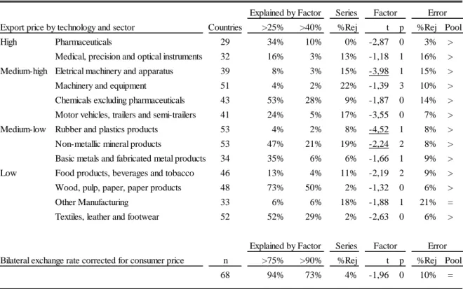
Table 3 shows results without the time trend. The general picture is much like before, with the exception of a larger proportion of non-stationary idiosyncratic components. There is also disagreement on the integration order of common factors for two
Table 3. PANIC test for unit root; only constant included 39 time periods
Series
Export price by technology and sector Countries >25% >40% %Rej t p %Rej Pool
High Pharmaceuticals 29 34% 10% 0% -2,87 0 3% >
Medical, precision and optical instruments 32 16% 3% 13% -1,18 1 16% >
Medium-high Eletrical machinery and apparatus 39 8% 3% 15% -3,98 1 15% >
Machinery and equipment 51 4% 2% 22% -1,39 3 10% >
Chemicals excluding pharmaceuticals 43 53% 28% 9% -1,87 0 14% >
Motor vehicles, trailers and semi-trailers 41 24% 5% 17% -3,55 0 7% >
Medium-low Rubber and plastics products 53 4% 2% 8% -4,52 1 8% >
Non-metallic mineral products 53 47% 21% 19% -2,24 2 8% >
Basic metals and fabricated metal products 34 35% 6% 6% -1,66 1 9% >
Low Food products, beverages and tobacco 46 13% 4% 11% -2,19 2 9% >
Wood, pulp, paper, paper products 48 73% 50% 2% -1,32 0 6% >
Other Manufacturing 33 6% 6% 18% -1,88 1 21% =
Textiles, leather and footwear 52 52% 29% 2% -2,63 0 6% >
Series
Bilateral exchange rate corrected for consumer price n >75% >90% %Rej t p %Rej Pool
68 94% 73% 4% -1,96 0 10% =
Notes: (i) "Explained by Factor" is the fraction of n countries where the common factor explains at least 25, 40, 75 or 90 percent of the variation. (ii) "%Rej" is the fraction of the original or error series for which the unit-root hypothesis is rejected. (iii) The Dickey-Fuller t-test statistic and lag order are shown only for the common factor, and rejection is indicated be an underline. (iv) A greater Explained by Factor Factor Error
16 of the industrial sectors. But common factors still account for very little of the variation in the export price series, the opposite being the case for the exchange rate series.
4. Results on panel cointegration
We present coefficient estimates for the partial effect of the bilateral exchange rate on export price controlling for marginal cost. The most direct way of attributing meaning to this coefficient is through the first order condition for the profit maximization problem of a representative domestic firm from a given industry exporting to several destinations. The bilateral exchange rate enters the first-order condition of the respective destination, and may be interpreted as a demand or cost shift. Comparative statics imply mark-up adjustments specific to each market. Equilibrium effects may be incorporated implicitly in residual demand curves or explicitly in additional first order conditions. The econometric model proposed here is a log-linear approximation of the bilateral exchange rate comparative statics effect which implicitly assumes small higher order effects.
There are many ways to model this formally. The essential point, though, is variable demand elasticity along the demand curves. Kneeter (1989) presents a simple model for an arbitrary residual demand function. Dornbush (1987) explores the residual demands that emerge from different market structures. Atkeson and Burstein (2008) take demand elasticity as a function of market share and preferences for variety. The structural interpretation is essentially static, but the inclusion of a time trend will hopefully capture changes in equilibrium market structure. The next section discusses structural models in greater detail to anchor theoretical expectations on microeconomic fundamentals.
The econometric model for the panel data set for an arbitrary sector is,
pit = dit + eit + i MgCt + uit (2)
17 order one; this is in conformity with results from the last section. The error term uit may be at most weakly dependent on the time and the cross-section dimension.
The coefficient measures the partial effect of the bilateral real exchange rate, and is the parameter we are interested at. This coefficient is pooled across destination countries. As a consequence, in case there is significant heterogeneity of firm behavior across markets, the parameter actually represents an average effect, as noted by Philips and Moon (1996). The coefficient i measures the partial effect of the marginal cost. It is country specific, which allows for different compositions of export bundles to different countries, or any other reason for some degree of freedom in the assessment of marginal cost relevant for a destination country.
The model follows very closely Bai, Kao and Ng (2009), with the marginal cost trend in equation (2) standing for a common factor in their terminology. Given our desired structural interpretation, we did not use information criterion to set the number of common factors, just fixing it at one as in equation (2). Except for low-technology goods, we argue below results are not very sensitive to this assumption. As for the deterministic term, we have tried the model with and without a deterministic trend. The qualitative results are reasonably close to each other, but with the trend better adhering to the data. The estimation method once again uses principal components to extract the common factor implicit in the export price indexes. Since this allows one to recover the marginal cost trend only up to a linear transformation, there is no expected sign pattern on i‟s coefficients. For this reason, we will not emphasize these estimates, rather concentrating on the exchange rate effect.
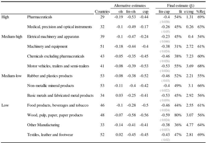
As a matter of comparison, we also estimated two alternative models. The first is
Kneeter‟s specification, for which variables enter in first-difference and the marginal cost trend enter as a fixed time effect (differencing is necessary, given our results on unit-roots from the previous section). The second is Philips and Moon (1996) fully modified estimator, which amounts to model (2) with i‟s restricted to be zero; that is, disregarding
any cross-sectional dependency.
18 Like the previous empirical literature, Kneeter‟s specification leads to very high levels of pass-through and to a few counterintuitive signs. The Philips and Moon specification appears to be more sensible, but it does not account for cross-sectional dependency (which is very likely given the results from the previous section), and it does not attempt to control for marginal cost, which is necessary for an economic interpretation.
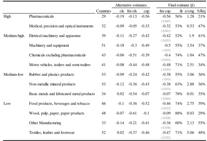
The estimator from Bai, Kao and Ng addresses both issues simultaneously. Their fully modified continuously updated estimator, which has a normal asymptotic distribution, is reported on the fifth column, with standard errors in the column next to it. All coefficients are negative at any reasonable significance level. The degree of pass-through implied by the coefficients is much more plausible then the one implied by previous methods. Comparing the fifth and the third column, we see that cross-sectional dependence is an important issue for most of the sectors. Now comparing the fifth with the fourth
Table 4. Panel cointegration results; one factor; constant and time-trend included 39 time periods
Countries ols fm-ols cup fm-cup fit e/cmg %Rej
High Pharmaceuticals 29 -0.19 -0.53 -0.44 -0.4 54% 1.31 69%
( 0.038)
Medical, precision and optical instruments 32 -0.1 -0.49 -0.17 -0.26 45% 0.26 63% ( 0.05)
Medium-high Eletrical machinery and apparatus 39 -0.1 -0.47 -0.24 -0.23 45% 0.4 54% ( 0.046)
Machinery and equipment 51 -0.18 -0.44 -0.4 -0.38 31% 2.72 61%
( 0.024)
Chemicals excluding pharmaceuticals 43 -0.05 -0.35 -0.45 -0.46 38% 7.23 60% ( 0.026)
Motor vehicles, trailers and semi-trailers 41 -0.08 -0.39 -0.53 -0.53 55% 3.69 68% ( 0.026)
Medium-low Rubber and plastics products 53 -0.08 -0.38 -0.52 -0.46 52% 2.21 55% ( 0.03)
Non-metallic mineral products 53 -0.11 -0.4 -0.42 -0.4 49% 3.1 66% ( 0.022)
Basic metals and fabricated metal products 34 0.03 -0.25 -0.41 -0.53 45% 2.92 56% ( 0.039)
Low Food products, beverages and tobacco 46 -0.1 -0.28 -0.5 -0.46 44% 2.55 61% ( 0.024)
Wood, pulp, paper, paper products 48 -0.07 -0.58 -0.56 -0.59 80% 3.07 56% ( 0.024)
Other Manufacturing 33 -0.14 -0.41 -0.41 -0.38 36% 4.77 64%
( 0.033)
Textiles, leather and footwear 52 0.02 -0.45 -0.45 -0.43 47% 2.81 69% ( 0.02)
Notes: (i) "ols" is the estimator from Kneeter. (ii) "fm-ols" is the estimator from Philips and Moon. (iii) "cup" is the continously updated estimator from Bai, Kai and Ng. (iv) "cup-fm" is the fully modified version of the last estimator, with standard error in parentheses. (v) The fit is the median explained variance among destination countries. (vi) The "e/cmg" is the median ratio of variances of the exchange rate effect and the marginal cost effect. (vii) "%Rej" is the fraction of rejections of the unit-root null aplied to model residuals of each country in the sector.
19 column, we notice that endogeneity of regressors, probably of the common marginal cost trend, may be an issue in some industrial sectors. Given the superior performance of the fully modified continuously updated estimator in the Monte Carlo experiments conducted by Bai, Kao and Ng (2009), we take this as our final estimator, and all the other summary measures in Table 4 take this reference point.
The “fit” column on Table 4 refers to the median explained variance, where the
median is taken with respect to export destination countries. The simple model with exchange rates and a single common factor as regressors explains about 50% of the variation in the export price data. Most of the explained variation comes from the exchange rate effects. This can be read from the next to last column, where it is shown the median
Table 5. Panel cointegration results; one factor; only constant included 39 time periods
Countries ols fm-ols cup fm-cup fit e/cmg %Rej
High Pharmaceuticals 29 -0.19 -0.13 -0.56 -0.56 56% 1.28 21%
( 0.045)
Medical, precision and optical instruments 32 -0.09 -0.05 -0.33 -0.32 53% 0.53 47% ( 0.041)
Medium-high Eletrical machinery and apparatus 39 -0.11 -0.27 -0.42 -0.42 52% 1.9 41% ( 0.033)
Machinery and equipment 51 -0.18 -0.3 -0.49 -0.5 55% 3.54 37%
( 0.03)
Chemicals excluding pharmaceuticals 43 -0.06 -0.51 -0.39 -0.4 74% 1.04 47% ( 0.033)
Motor vehicles, trailers and semi-trailers 41 -0.08 -0.44 -0.48 -0.48 71% 2.51 34% ( 0.039)
Medium-low Rubber and plastics products 53 -0.09 -0.24 -0.42 -0.38 55% 3.06 36% ( 0.03)
Non-metallic mineral products 53 -0.12 -0.36 -0.43 -0.38 63% 2.88 36% ( 0.033)
Basic metals and fabricated metal products 34 0.02 -0.54 -0.07 -0.07 78% 0.01 35% ( 0.064)
Low Food products, beverages and tobacco 46 -0.1 -0.36 -0.52 -0.46 74% 2.75 39% ( 0.032)
Wood, pulp, paper, paper products 48 -0.07 -0.61 -0.1 -0.09 88% 0.03 29% ( 0.038)
Other Manufacturing 33 -0.14 -0.21 -0.41 -0.36 60% 2.13 55%
( 0.038)
Textiles, leather and footwear 52 0.02 -0.37 -0.46 -0.47 71% 5.06 48% ( 0.022)
Alternative estimates Final estimate ()
20 ratio of the variation due to exchange rate and the variation due to the common factor. The last column presents the fraction of countries residual series where the unit-root null is rejected. Critical values were obtained admitting three cointegrated variables. Given the low power of single-series tests, there is very strong evidence that residuals are stationary. This means the relationship summarized by the coefficient is not spurious.
Table 5 shows results without the time-trend and can be similarly interpreted. Comparing with the previous table, the fully modified continuously updated estimator is larger in absolute value in most sectors but follows the previous estimates closely. There are only two abnormal sectors for which the full pass-through hypothesis cannot be rejected and for which the exchange rate effect contributes to very little of price variation. The
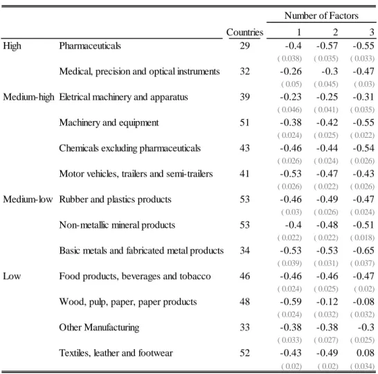
Table 6. Sensitivity of parameter estimate () to the number of factors
Countries 1 2 3
High Pharmaceuticals 29 -0.4 -0.57 -0.55
( 0.038) ( 0.035) ( 0.033)
Medical, precision and optical instruments 32 -0.26 -0.3 -0.47
( 0.05) ( 0.045) ( 0.03)
Medium-high Eletrical machinery and apparatus 39 -0.23 -0.25 -0.31
( 0.046) ( 0.041) ( 0.035)
Machinery and equipment 51 -0.38 -0.42 -0.55
( 0.024) ( 0.025) ( 0.022)
Chemicals excluding pharmaceuticals 43 -0.46 -0.44 -0.54
( 0.026) ( 0.024) ( 0.026)
Motor vehicles, trailers and semi-trailers 41 -0.53 -0.47 -0.43
( 0.026) ( 0.022) ( 0.026)
Medium-low Rubber and plastics products 53 -0.46 -0.49 -0.47
( 0.03) ( 0.026) ( 0.024)
Non-metallic mineral products 53 -0.4 -0.48 -0.51
( 0.022) ( 0.022) ( 0.018)
Basic metals and fabricated metal products 34 -0.53 -0.53 -0.65
( 0.039) ( 0.031) ( 0.037)
Low Food products, beverages and tobacco 46 -0.46 -0.46 -0.47
( 0.024) ( 0.025) ( 0.02)
Wood, pulp, paper, paper products 48 -0.59 -0.12 -0.08
( 0.024) ( 0.032) ( 0.032)
Other Manufacturing 33 -0.38 -0.38 -0.3
( 0.033) ( 0.027) ( 0.025)
Textiles, leather and footwear 52 -0.43 -0.49 0.08
( 0.02) ( 0.02) ( 0.034)
Number of Factors
21 Philips and Moon estimator does a much poorer job than before, indicating the greater importance of cross sectional dependency when no time-trend is included. Finally, the model residuals appear to be much less stationary then the previous case, suggesting that spurious regression may now be a serious issue. Overall, there is enough evidence to conclude that the time-trend specification is the superior one. As suggested before, it is likely that other permanent shock disturb the long-run relationship of interest, and the deterministic trend proxies for them. From this point on, we consider only the coefficients estimated under the assumption of country specific constant and time-trend.
The inclusion of additional common factors preserves most of the results, apart from low technology sectors. Information criteria based on Bai and Ng (2002) provide no strong indication on the number of factors, with one or three factors being the preferred choice depending on the criteria; in any case, information criteria do not have robust properties in small finite samples. Table 6 reports the coefficient estimates and standard errors with as much as three common factors. Except for low technology ones where the single factor assumption seems to be essential, the pattern of results is fairly robust to the assumption. Without clear indication to the contrary by information criteria, parsimony and structural interpretation lead us to impose the single factor specification for all sectors.
5. Discussion
The main motivation for estimating long-run parameters was to improve on the previous panel literature, possibly obtaining a clearer picture on pricing-to-market behavior. The long-run coefficients are indeed much less dispersed then short-run analogues of the traditional panel literature reviewed before. Additionally, the sign pattern of negative mark-up effects significantly different from zero is more aligned with the aggregate evidence of incomplete pass-through which motivated the literature in the first place5. In this section, we show the estimated coefficients have interesting patterns and connections with microeconomic fundamentals.
5
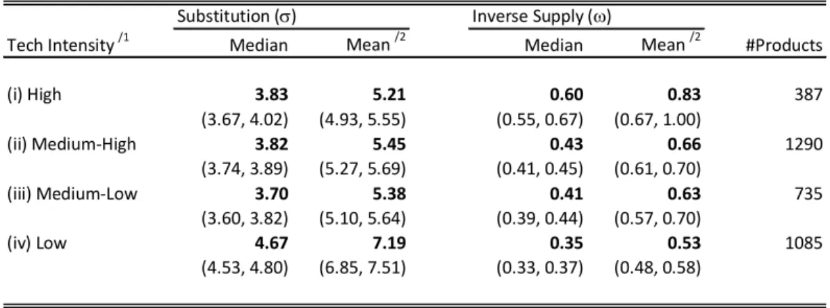
22 The industrial classification scheme used in the paper is essentially based on the research and development activities in each industry which may have connections with preference and market structure parameters. High technology sectors are constantly developing new product varieties to attend very specific consumer needs - for example, consumers of medical appliances and pharmaceuticals very often have few substitution possibilities. As for the market, competition is not expected to be high if measured by the average mark-ups in the industry which reflects large market shares among key participants. On the opposite extreme, low technology industries represent consolidated business with a large number of players offering very substitutable commodities. There is indeed econometric evidence supporting this informal argument. Barroso (2009) found technological intensity is positively associated with product differentiation and supply elasticity.
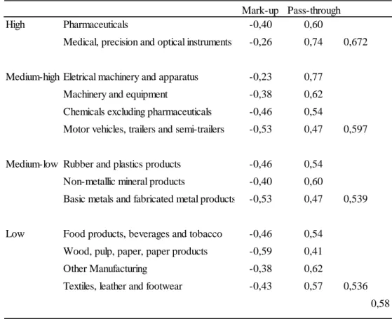
Table 7. Long-run margin and pass-through effects by technological intensity
Mark-up Pass-through
High Pharmaceuticals -0,40 0,60
Medical, precision and optical instruments -0,26 0,74 0,672
Medium-high Eletrical machinery and apparatus -0,23 0,77
Machinery and equipment -0,38 0,62
Chemicals excluding pharmaceuticals -0,46 0,54
Motor vehicles, trailers and semi-trailers -0,53 0,47 0,597
Medium-low Rubber and plastics products -0,46 0,54
Non-metallic mineral products -0,40 0,60
Basic metals and fabricated metal products -0,53 0,47 0,539
Low Food products, beverages and tobacco -0,46 0,54
Wood, pulp, paper, paper products -0,59 0,41
Other Manufacturing -0,38 0,62
Textiles, leather and footwear -0,43 0,57 0,536
0,58
23 Table 7 calculates simple averages of pass-through coefficients for each level of technological intensity. At least for this sample, it appears that pass-through is increasing with technology. It is suitable to add some theoretical underpinning to these observations. For that matter, is not hard to argue that high substitution and low shares lead to lower pass-through. In Dornbush (1987), high substitution is complementary to competitors‟ responses to expected aggregate price changes in the industry, and each firm is forced to adjust markups more strongly. Atkeson and Burstein (2008) show that mark-ups are sensitive to market-shares, the more so for higher elasticities of substitution. Since mark-shares reflect differences in marginal costs the result follows. In both models, high market shares increases the influence on the sector price and therefore the pass-through that can be implemented. Of course, the actual details of the arguments leading to these interactions depend on the precise market structure and demand schedule assumed by the authors. But the pattern suggested by Table 7 and the underlying connection with microeconomic fundamentals argued for in the last paragraph both support models with this properties.
24 6. Conclusion
There is strong evidence of long-run pricing-to-market behavior by Brazilian exporters. Approximately 58% of an exchange rate appreciation would be passed-through to foreign consumer prices, with Brazilian exporters absorbing a 42% loss through reduced mark-ups. The degree of pass-through is positively related to the technological intensity of the industrial sector, a sensible pattern given the lower substitution between product varieties in high technology sectors. These results cannot be attributed to sticky-price constraints which by definition are not binding in the long-run. Therefore, the significant long-run effects support market structure explanations of incomplete pass-through and deviations from purchasing power parity, with possible normative consequences for trade and exchange rate policy.
References
ATKESON, Andrew and BURSTEIN, Ariel. 2008. Pricing-to-market, trade costs, and international relative prices. American Economic Review, 98:5, 1998-2031
BAI, Jushan; KAO, Chihwa and NG, Serena. 2009. Panel Cointegration with Global Stochastic Trends. Journal of Econometrics, 149, 1.
BAI, Jushan and NG, Serena. 2002. Determining the number of factors in approximate factor models. Econometrica, 70, 1.
BAI, Jushan and NG, Serena. 2004. A PANIC Attack on Unit Roots and Cointegration.
Econometrica, 72, 4.
BUGAMELLI, Matteo and TADESCHI, Roberto. 2008. Pricing-to-Market and Market Structure. Oxford Bulletin of Economics and Statistics, 70, 2.
DORNBUSH, Rudiger. 1997. Exchange Rates and Prices. The American Economic Review, 77, 1.
25 HATEMI-J , Abdulnasser and IRANDOUST, Manuchehr. 2004. Is Pricing to Market Behavior a Long-Run Phenomenon? A Non-Stationary Panel Analysis. Empirica 31: 55– 67.
KNETTER, Michael. 1989. Price Discrimination by U.S. and German Exporters. The
American Economic Review, 79, 1.
KRUGMAN, Paul. 1986. Pricing-to-market when the exchange rate changes. NBER
Working Paper, 1926.
MÉJAN, Isabelle. 2004. Exchange rate movements and export prices: an empirical analysis. CREST Working Paper 2004-27.
OTANI, Akira. 2002. Pricing-to-market and the international monetary policy transmission: the new open-economy macroeconomics approach. Monetary and Economics Studies from
the Bank of Japan.
PHILLIPS, Peter and MOON, Hyungsik. 1999. Linear regression limit theory for nonstationary panel data. Econometrica, 67, 5.
RAVN, Morten. 2001. Imperfect competition and Prices in a Dynamic Trade Model with Comparative Advantage. CEPR Working Paper.
SUTHERLAND, Alan. 2005. Incomplete pass-through and the welfare effects of exchange rate variability. Journal of International Economics, 65, 375– 399
TAKAGI, Shinji and YOSHIDA, Yushi. 2001. Exchange rate movements and tradable goods prices in East Asia: an analysis based on Japanese customs data. IMF Staff Papers, 48, 2.
26
Gains from Imported
Varieties in the Brazilian Economy
Abstract
This paper estimates welfare gains from new varieties of imported goods in Brazil since the 90s taking into full account preference and technology heterogeneity, in the sense of how easily substitutable are varieties of different goods to each other. Elasticities of substitution are estimated for a broad spectrum of consumer and intermediate goods using Feenstra (1994) method, which explores heteroscedasticity in the panel dimension to obtain identification of the structural parameters. An extension of Broda and Weistein (2006) aggregation model allowed productivity effects of intermediate goods to have an impact on welfare calculations. The welfare calculation points to significant gains from new varieties of imported goods, of the order of 0.5% of gross domestic product, most of which due to intermediate goods. Estimated elasticities of substitution are shown to have systematic relations to market structure indicators. They also point to significant aggregation bias in the literature‟s estimates of aggregate elasticities of substitution and aggregate price-indexes.
JEL Classification: C52, D60, F12, F40
27 1. Introduction
The greater availability of varieties is an important source of gains from trade, particularly when consumers or firms are less willing to substitute one variety for another [Krugman (1978), Ethier (1982)]. Indeed, elasticities of substitution between goods are crucial inputs for most positive and normative questions in open economy macroeconomics and international trade. They are usually estimated for broad categories, thus relying on strong homogeneity restrictions. Since the microeconomic evidence points to heterogeneity, some authors [Broda and Weinstein (2006), Imbs and Méjan (2008)] have been revisiting the aggregate exercises from more solid foundations. Building on ideas by Feenstra (1994), the new approach obtains sensible estimates of product level elasticities of substitution within a theoretical model that allows straightforward aggregation. This paper follows the approach to answer the question: what was the welfare impact from the changing varieties of imported goods since the opening up of the Brazilian economy in the 90s? Also of interest is if there are any discernible patterns in the elasticities of substitution estimates underlying the welfare impact calculations and what are their implications for aggregate import elasticities of substitution, relevant for counter-factual analysis.
28 commodities; the point was to evaluate if price effects in trade equations were underestimated due to unnoticed variation in the actual price index, which was the result for some of the goods analyzed by the author.
The method was extended to the many commodities case by Broda and Weinstein (2006), who were able to calculate an aggregate import price index with the appropriate correction for variety change. Note that absolutely new goods pose an obstacle to
Feenstra‟s approach, which handles changing varieties only within goods categories with some trade data in both periods under consideration. Broda and Weinstein circumvent the issue by aggregating goods in broad categories whenever necessary. The authors also embed the import decision in the wider consumer decision problem, and are thus able to make aggregate welfare inferences. The convenient price index formula actually allowed the authors to calculate the compensating variation to improved variety, that is, a money metric equivalent of the welfare improvement obtained with the expanded set of goods. The gains from variety for the United States from 1972 to 2001 are estimated as 2.6 percent of 2001 income. An important shortfall in these calculations, acknowledged by the authors, is the bundling of commodities in a single consumer good category. This means gains from variety of imported intermediate and capital goods receive no separate treatment.
29 substitution, estimated with the usual time-series methods, was imputed to be relatively low. Rutherford and Tarr (2002) build a model with capital accumulation where the transition dynamics between steady-states after a 10% import tariff cut in intermediate goods leads, in the very long run, to a 10% welfare increase in present value terms, mainly due to the entry of new intermediate producers.
The results from this literature depend on estimates of aggregate elasticities of substitution between goods from home and foreign countries, the country of origin being the usual concept of variety. Most econometric methods indentify the parameters of interest from the responsiveness of aggregate quantities to changes in aggregate prices, which usually results in very low elasticities of substitution relative to microeconomic studies. Imbs and Méjan (2008) document aggregation bias originated from the positive correlation between elasticities of substitution and shares in the enclosing category. They argue that aggregate elasticities of substitution relevant for representative agent models are actually much larger than the usual estimates6. Thus, the gains from new imported varieties derived from general equilibrium models with endogenous introduction of new goods may be lower than previously thought.
This paper makes several contributions to the literature. An important advance is to extend Broda and Weinstein (2006) method to account for the productivity effect of importing new kinds of intermediate goods. The extension is particularly relevant for a developing country such as Brazil in the nineties. The paper advocates a chained index method which reduces aggregation due to the absolutely new good problem mentioned above and allows more accurate figures on year-to-year gains from trade. On the
econometric side, an improvement in robustness is obtained from coupling Feenstra‟s
estimator and a parametric bootstrap procedure. Given the large number of models and the likely presence of undetected outliers, it is important to have a robust procedure. The estimated elasticities of substitution are confronted with known patterns documented by Broda and Weinstein (2006); also, an attempt is made to uncover new regularities. The paper clarifies the relation between the welfare gain specification and Imbs and Méjan
6
30 (2008) specification, thus allowing for consistent aggregation of estimated elasticities of substitution.
There are a number of substantive contributions, more closely concerned with Brazil, with potential application in open economy macroeconomic research. These range from aggregate import price index corrected for the introduction of new goods, to aggregate elasticities of substitution for imports free from aggregation bias. The elasticities estimates are particularly relevant for calibrating general equilibrium models of the Brazilian economy. As an appraisal of this estimates, the paper contrasts them with the available state of the art time-series estimates of Armington elasticities. In addition, disaggregated elasticities parameters themselves are important inputs for many kinds of frontier research - for example, Chaney (2008) notes that the elasticity of substitution provides conflicting incentives for the extensive and intensive margin of bilateral trade flows, and used Broda and Weinstein (2006) estimates to explore the issue empirically. The main substantive contribution, though, is a money metric measure of the welfare gains from new varieties of imported goods for the Brazilian Economy in the 1989 to 2008 period, which has not been addressed by previous research.
2. Economy
2.1. Preferences and Technology
31 Imported consumer good k may be available in varieties iI, which refer to foreign
countries. Preferences over the consumption of varieties (mkit)iI of imported good k at time period t are represented by the function
(1)
where k is the constant elasticity of substitution for varieties of good k and bkit is the time varying quality parameter for variety i of good k. Moving up, preferences over the consumption of sets of varieties of imported goods are represented, in terms of consumption aggregates (mkt)kK, by the function
(2)
where is the elasticity of substitution for imported goods. Finally, preferences over all goods and varieties are defined in terms of the import aggregator mt and an arbitrary
domestic goods aggregator dt,
(3)
32 separable inputs in the economy gross production function and the set of varieties for each good are also separable from each other.
Each imported intermediate good j may be available in varieties iI. The economy
bundles imported intermediate varieties (xjit)iI in period t to produce the aggregate intermediate good xjt using the production function
(4)
where j is the constant elasticity of substitution for varieties of good j and ajit is the time varying quality parameter for variety i of good j. The intermediate goods (xjt)jJ are further aggregated into a single imported intermediate good xt with production function
(5)
where is the constant elasticity of substitution for intermediate goods. The economy takes as input this imported intermediate good xt, an aggregate of domestic intermediate goods zt and other primary factors lt to obtain gross income with the production function
(6)
Home intermediate goods are produced from primary factors with constant returns to scale.
2.2. Equivalent Variation
33 The representative consumer faces prices pt=(pkt) kK=({pkit:iIkt}) kK, where IktI is the subset of countries from which good k may be imported in period t. The set of available varieties in each period is taken as given. From equation (1), the unit cost function associated with consumer good k is
(7)
The exact price index for good k given prices and consumer choices, supposing constant quality parameters b and a fixed set of available varieties , is the well known Sato-Vartia exact price index,
(8)
where wkit is the normalized log-change share in the good‟s expenditure defined by
(9)
Let Ik be a subset of varieties from good k available in period t and t-1, for which quality parameters have remained constant. We may refer to this subset as the common varieties. As shown by Feenstra (1994), the exact price index for gook k is given by
(10a)
34
(10b)
The intuition for the result is taking the prices of unavailable varieties to infinity in the ratio of unit costs with different sets of varieties; the decomposition in equation (10) then follows naturally. As is evident in the formula, new varieties reduce the lambda ratio and therefore the exact price index; small elasticities of substitution and large shares of these varieties in total consumption both contribute to a larger reduction.
Aggregation is straightforward. Indeed, as in Broda and Weinstein (2006), suppose there is a collection IK=(Ik)kK of subsets of common varieties for each good in a constant set of goods K. Apply the Sato-Vartia exact price index to the aggregate consumption of imported goods mt shown in equation (2). Now, the unit cost function is the correct concept
of aggregate import price; and we obtain the exact price index number for imported goods:
(11a)
where wkt is the normalized log-change share in import expenditure, and the arguments in the price index formula for each good where suppressed. At times, it will be convenient to use the more compact notation
(11b)
By the same argument, the aggregate consumer price index associated with equation (3) is
(12)
where wd and wm are log-change share of domestic and imported goods in consumption
35 Proposition 1 [Feenstra (1994), Broda and Weinstein (2006)]. Suppose there is a common set of varieties Ik. Then the exact price index for good k is given by (10). If in
addition there is a collection of common varieties IK=(Ik)kK , then the exact aggregate price index is given by (11).
The firm‟s cost minimization problem for the production of the composite intermediate good is entirely analogous to the consumer problem. From Propostion 1, with the evident notation, the exact price index for imported intermediate goods is given by
(13)
To obtain the aggregate price index for the economy´s gross output, apply the usual Cobb-Douglas index,
(14)
Now, total production costs are equal to unit costs times production. Therefore,
(15)
We have all the ingredients to compute the equivalent variation. Indeed given consumer income in period t is , the equivalent variation relative to the initial period income is
(16)
36 The third equality used the production functions defined above so that z may be eliminated from the income ratio. Just divide the numerator and denominator by and use Cobb-Douglas for final goods, linearity on labor for intermediate goods, as labor as numeraire. To emphasize changes available varieties, rewrite the expression as
(17)
where depends only on the collection of common varieties and the last term is a measure of the welfare impact of new varieties.
Proposition 2. The equivalent variation may be decomposed in two terms, one of them measuring the welfare impact of variety change, as in equation (17).
The welfare measure just derived depends on the elasticity of substitution for many
disaggregated goods. To estimate these parameters, the paper applies Feenstra‟s (1994)
method, briefly reviewed in next section. We take some time to show the method is robust to tariffs and exchange rate pass-through decisions by firms.
3. Identification
From the cost minimization problems faced by consumers and firms, demand at period t for the country/variety i of a particular good k may be written in terms of their share in expenditure,
(18)