FUNDAÇÃO GETULIO VARGAS
ESCOLA de PÓS-GRADUAÇÃO em ECONOMIA
Lira Rocha da Mota
The Market for Borrowing Securities in
Brazil
Lira Rocha da Mota
The Market for Borrowing Securities in
Brazil
Dissertação para obtenção do grau de mestre apresentada à Escola de Pós-Grauação em Economia
Área de concentração: Finanças
Orientador: Marco Antônio Bonomo
Agradecimentos
Fragmento Oda al Mar
Todo lo arreglaremos poco a poco: te obligaremos, mar, te obligaremos, tierra, a hacer milagros, porque en nosotros mismos, en la lucha, está el pez, está el pan, está el milagro.
Abstract
We report the results of an exploratory data analysis of the Brazilian securities lending market. The analysis is performed over the full historical data set of each individual loan offer and loan contract negotiated between January 2007 and August 2013. We give a quantitative description of volume and loan fee trends and fee dependence on asset characteristics. We also unveil new stylized facts specific to the Brazilian market on market access asymmetries between different types of investors. The emerging picture is that the Brazilian securities lending market is a com-plex environment with specific frictions and strong asymmetries among players. In particular, we describe a tax arbitrage operation performed by domestic mutual funds which generates a significant distortion in the data. In one such event, we estimate additional aggregate profits of 24.25 million Reais (around 10 million Dollars).
List of Figures
2.1 Market Diagram . . . 5
4.1 Loan Balance: Lenders . . . 12
4.2 Loan Balance: Borrowers . . . 13
4.3 Distribution of Loan Fees By Firms: 2007-2013 . . . 14
4.4 Distribution of Loan Fees By Firms by Year . . . 15
4.5 Median of Loan Fees Through Time . . . 15
4.6 Mutual Funds Fee Relative Spread: Lender . . . 21
4.7 Mutual Funds Fee Relative Spread: Borrower . . . 21
5.1 Time Series: VALE5 . . . 25
5.2 Time Series: PETR4 . . . 26
5.3 Time Series: AMBV4 . . . 27
5.4 Time Series: OGXP3 . . . 28
5.5 IoNE Settlement Date: AMBV4 . . . 29
5.6 IoNE Settlement Date: VALE5 . . . 30
5.7 IoNE Settlement Date: PETR4 . . . 30
5.8 Lending Fee around IoNE Settlement date Date . . . 31
5.9 PETR4 Contracts . . . 32
List of Tables
2.1 Taxation Table . . . 8
4.1 Shares in Equity Market . . . 13
4.2 Fee Distribution by Firms . . . 14
4.3 Loan Fee (%) by Market Cap, Turnover and Volatility . . . 17
4.4 Loan Balance (mi) by Market Cap, Turnover and Volatility . . . 18
4.5 Loan Fee Panel Regressions . . . 19
4.6 Loan Balance Panel Regressions . . . 19
4.7 Presence of Recall Right . . . 22
4.8 Important Securities: Average Fee (%) . . . 22
4.9 Important Securities - Number of Contracts (millions) . . . 23
5.1 Profit Distribution Analysis: Foreign Investors . . . 33
Contents
1 Introduction 1
2 Market Description 4
2.1 Little Bit of History . . . 4
2.2 Mechanism Description . . . 4
2.3 Players . . . 5
2.3.1 BM&FBovespa . . . 5
2.3.2 Final Investors . . . 6
2.3.3 Brokers . . . 6
2.4 Contract Specifications . . . 6
2.4.1 Right of Recall . . . 6
2.4.2 Reference Price . . . 6
2.4.3 Directional Offers . . . 6
2.4.4 Offer’s Expiry Date . . . 7
2.4.5 Renewal . . . 7
2.4.6 Grace Period . . . 7
2.5 Regulation . . . 7
2.6 Taxes and Transactions Fees . . . 7
2.7 Automatic Loan . . . 8
3 Database Description 9 3.1 Offers Database . . . 9
3.2 Contracts Database . . . 10
3.3 Liquidation Database . . . 10
3.4 Complementary Databases . . . 10
4 Empirical Facts about the Loan Market 11 4.1 Volume, Players and Fees . . . 11
4.2 Fee Dependence . . . 16
4.3 Players Analysis . . . 20
4.4 Right of Recall . . . 22
5 Tax Arbitrage 24 5.1 Case Study: PETR4 . . . 31
6 Conclusion 34
Chapter 1
Introduction
The impact of short selling constrains on financial markets has been extensively analyzed in the economic literature. In his pioneering work, Miller (1977) explored the relation between short selling restrictions, risk and divergence of opinion in a market with investors with dif-fering estimates on expected returns. Miller’s overvaluation hypothesis is that short sale con-straints can prevent negative information or opinions from being reflected into stock prices, leading to overpriced stocks. Other authors gave important contributions to the field, and to-day there is a rich literature on the implications of short selling constrains and, more widely, limits on arbitrage. (e.g., Diamond and Verrecchia (1987), Harrison and Kreps (1978), Hong and Stein (2003), Hong et al. (2006)).
The mechanism of short sell is intimately related to the securities lending market:
“A short sale is the sale of a security that the seller does not own or that the seller owns but does not deliver. In order to deliver the security to the purchaser, the short seller will borrow the security, typically from a broker-dealer or an institutional investor. The short seller later closes out the position by returning the security to the lender, typically by purchasing equivalent securities on the open market.”
SEC Concept Release No. 34-42037
In this sense, understanding the lending market is a prerogative to understand the origins of short selling constrains. Finance theory often makes strong assumptions about the ability to borrow and short arbitrarily large amounts of stocks, sometimes ignoring the operation costs or considering them as fixed. However, when securities loan market is analyzed in more detail, it is easy to recognize its complexity. D’Avolio (2002), for example, argues that the loan market should be inserted into a supply and demand framework with possible economics frictions and rejects the idea of treating loan fees as ordinary “transactions costs”. Duffie et al. (2002) provides related work with a multi-period model of the equity loan market that emphasizes the search process faced by borrowers and lenders and their consequences on loan fee.
BM&FBovespa, the only stock exchange presently operating in Brazil, turning the lending mar-ket into a centralized marmar-ket. The centralized framework mitigates data aggregation problems encountered in many short selling studies because BM&FBovespa gathers information of the market as whole.
In this thesis we perform a detailed empirical study about the security lending market in Brazil. The study is based on the complete dataset 1 of loan offers and loan contracts made
between January 2007 and June 2013. The key points of the analysis are the identification of: (i) volume increasing and loan fee decreasing trends; (ii) fee positive dependence on turnover, volatility and negative dependence on market capitalization; (iii) market access asymmetries among different types of investors (iv) price discount when considering contracts that guaran-tees the right of recall; (v) tax arbitrage strategies involving the lending market. We also detail the mechanism of lending and borrowing stocks as well as the regulatory aspects. The aim is to identify drivers of the loan fee formation, and to understand possible abnormal market events. This unique analysis is made possible by the access to data regarding each individual loan contract and all contracts’ life-cycle, from the submission of the offer until the liquidation process. We also have access to information about the type of investor on both sides the loan contract, hence we can identify if the investor is a retail investor, hedge fund, foreign investor, commercial bank, etc.
Among other findings we describe an tax arbitrage opportunity that is associated with large loan fee and loan balance fluctuations. We calculated the exact profit obtained for player that could benefit themselves from this fiscal policymanoeuvrefor a specific example involving
PETR4. We arrived at the remarkable number of 24.25 million Reais (around 10 million Dollars) aggregate profit for just a single event. We believe that the analysis of this phenomenon is not only interesting in itself, but it is also of relevance for any further empirical study on the Brazil-ian lending market. The magnitude of the impact of interest payments on net equity on loan fees is so big that any econometric finding disregarding this phenomenon could potentially be spurious.
De-Losso et al. (2013) recently presented a work about the Brazilian lending market. They rely on similar econometric framework as Cohen et al. (2007) to assess the impact of short selling restriction on prices. Using data on the actual shifts of the lending supply curve of a set of 44 Brazilian stocks, they find evidence to confirm the original hypothesis of Miller (1977). In our work, whereas, we performed an exploratory data analysis of the complete Brazilian lending market. Relevant stylized facts emerged from the analysis, which, to my best knowledge, are new in the academic literature2. The objective here is to allow the reader to
gain a qualitative and quantitative understanding of the market as a whole.
The motivation to this thesis lies on the fact that lending market is witnessing a steady pro-cess of popularization and growth in Brazil. From January 2007 until August of 2013 the vol-ume lent increased five times, with an average annual volvol-ume growth of 23.5%. The monthly average of generated financial volume is equal to 3% of BM&FBovespa market capitalization. Nowadays, borrowing and short selling stocks is a wide-spread practice in the Brazilian finan-cial market. Buy side investors rely on this mechanism to perform directional trading strategies, hedging and pair trading3.
Short selling is also a widely discussed topic among policy makers. Up until now, there is no wide consensus on the consequences of short selling on financial market stability and price
1The dataset was kindly provided by BM&FBovespa
2Interviews with broker dealers and hedge funds operating in Brazil confirmed the likely hypothesis that,
de-spite the lack of quantitative data, those operating in the market do have a qualitative knowledge of some of the results presented in the paper.
3Pair trading is an arbitrage strategy of matching a long position with a short position in two stocks with
formation transparency. On one hand, short selling is considered an important mechanism to provide market liquidity and efficient price discovery, on the other, there are concerns that short selling practice may leverage sharp drops in prices, severely harming market sustainability.
Furthermore, our motivation to this research lies on the fact that discussion about short selling has gained renewed vigor with the 2008 and European crises. In the latest years, short selling restrictions have been implemented in different degrees across many countries. U.S., for example, adopted a very controversial policy when it temporarily banned short selling after Lehman Brothers filed for bankruptcy. Later on, several European countries temporarily or permanently banned short selling in an attempt to slow down falling stock prices. The true impact of these actions, although very hard to measure, has been the research subject of many economists (see, e.g., Beber and Pagano (2009), Boehmer et al. (2013))
Chapter 2
Market Description
One singularity of the Brazilian lending market is that all transactions have to go through the Brazilian Clearing and Depositary Corporation (CLBC). Relying on a centralized model that guarantees different mechanisms of control, lending securities configures a very regulated and complex market. Even though the lending market has become very attractive to all kind of investors, offshore borrowers still find it difficult to relate the Brazilian securities lending model back to the model with which U.S. and European beneficial owners and borrowers are familiar1. This chapter is dedicated to elucidate the Brazilian lending mechanisms and its
reg-ulatory system. We use as main reference the documentation available only in Portuguese in BM&FBovespa’s website2.
2.1 Little Bit of History
Securities lending operations in Brazil began in the seventies, when there were mainly pri-vate contracts provided by brokers and some custodian banks. In 1996, BM&FBovespa started offering a centralized stock lending service through a system called “Banco de Títulos” - BTC. Since then, the stock exchange is responsible for offering services of parties’ registration, risk control, settling and custody services, as well as publishing lending market information. Mo-tivated by the increasing demand for lending services, BM&FBovespa created an electronic platform where all parties can post their offers.
2.2 Mechanism Description
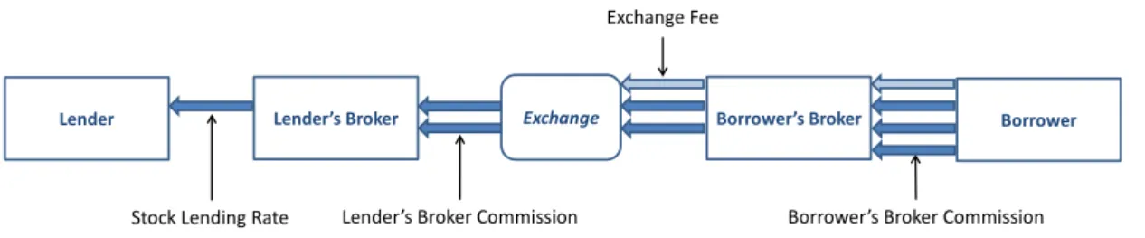
Securities lending involves a transfer of securities to a third party (the borrower). The bor-rower pays the lender an agreed annualized fee for the loan and is obliged to return the securi-ties in accordance to what was resisted in contract. The borrower becomes the temporary owner of the shares and detains all its rights, including votes. However, the borrower is obliged to pass over to the lender any dividends/interest payments and corporate actions that may arise. A typical lending operation involves the exchange and four different participants: the lender, the borrower, the lender’s broker and the borrower’s broker. The diagram bellow il-lustrates a typical loan contract:
1JPMorgan Regional Focus: Brazil (2011)
2BMF&Bovespa Security Lending System: http://www.bmfbovespa.com.br/pt-br/intros/
Lender Lender’s Broker Borrower’s Broker Borrower
Stock Lending Rate Le der’s Broker Co issio Borrower’s Broker Co issio
Exchange
Exchange Fee
Figure 2.1: Market Diagram
Payments among participants are determined by the the quantity of borrowed shares Q,
the number of working days the shares are borrowed du, and three fees: the lending raterl,
the lender’s broker commission raterlc and the borrower’s broker commissionrbc. When the
contract is liquidated, the following payments are performed:
• The borrower paysV F(rlc+rl+rbc)to the borrower’s broker;
• The borrower’s broker paysV F(rl+rbc)to the lender’s broker;
• The lender’s broker paysV F(rl)to the lender.
here,V F is given by:
V F(r) =Q×P ×
"
1 + r 100
252du
−1
#
(2.1)
whereQanddurefer to the specific trade, whileP is the price agreed before the trade3.
All securities issued by opened companies trading in BM&FBovespa are eligible for lending operation in the BTC system and the transference of securities is done in real time as soon as the contract is firmed.
2.3 Players
In this section we characterize the main players in a loan contract.
2.3.1 BM&FBovespa
The exchange acts as central counterparty for all trades. BM&FBovespa is responsible for controlling operational limits, calculating and managing collateral, guaranteeing proper liqui-dation and penalties, if necessary.
3Clearly, this is a stylized cash-flow payment scheme. The true liquidation process is managed by
2.3.2 Final Investors
Loan services are available to all investors registered in the exchange. Final investor must have custody agents to intermediate a loan contract, however, in respect of Brazilian regula-tion, custody agents in order to operate a loan contract must record in the BTC system their operations as well as the final investor required information: ID, type, accounts, etc.
2.3.3 Brokers
They are responsible to intermediate a loan contract on behalf of final investors. CVM 441 instruction makes broker intermediation mandatory in a loan contract. In order to lend clients shares, brokers must present a documentation where the final investor explicitly authorizes transferring his shares to a BTC account and releasing them to loan.
2.4 Contract Specifications
When an investor posts an offer (lender or borrower) in BTC the electronic platform he must specify some features that customizes the potential loan contract. Their abidance is guaranteed by the exchange. Those features are listed bellow:
2.4.1 Right of Recall
In U.S and European loan contracts, the borrower is usually obliged to return the securities on lender’s demand within the standard market settlement period. In Brazil, this is a cus-tomized feature of loan contract. If the lender chooses to maintain his right to recall, he may demand the shares at any time during the contract and delivery takes place in four business days. If the lender chooses to give up his right of recall, the contract ends at maturity or on borrower’s demand. Until 2011 contracts with right of recall were never performed, but since then this type of contract has become popular.
2.4.2 Reference Price
When contract is liquidated the payment is calculated over the financial value of the con-tract, P riceXQuantity. The price used in this calculation is agreed in contract. It can be the
VAWP4 of the day before contract was settled or VAWP of the day before contract was
liqui-dated. The most common type of contract uses as reference price the VAWP of the day before contract was settled, accounting for 98.7% of our sample.5
2.4.3 Directional Offers
It is possible to post directional offers in the BTC system. This is a type of offer where the terms are previously agreed between the parties. When a directional loan offer is sent to the BTC electronic system the offer is not public, as it would be if there was no prior agreement. The only participant who can actually see the offer is the broker to whom the offer was directed. In this case, the BTC system works just as a registration system. In our data-set directional and public offers are not differentiated. Directionalityis a confidential information, hence it is not
4Volume Weighted Average Price
5Since the presence of contracts that use as price reference the VAWP of the day before contract was liquidated
available in the database used in this thesis. Interviews with BM&FBovespa’s specialists, bro-ker dealers and institutional investors operating in the market strongly suggest that directional offers are the most common type of offers. In particular, all of our interviewees estimated that nowadays public offers account for less than 5% of the loan contracts.
2.4.4 Offer’s Expiry Date
When registering an offer, investors must specify expiry date that determines until when the offer is valid. Usually they respect a one month period.
2.4.5 Renewal
Investor must specify if there is a possibility to renew the loan contract after the maturity. In case of renewal, a new contract is created respecting the terms of the original one.
2.4.6 Grace Period
By regulation, the life of a loan contract must be at least one day. Lenders may specify in their offers a minimal period for borrower to hold the security, called glance period. After the grace period, lenders have the option to liquidate the contract at any time. The way to create a fixed time contract is to establish the grace period equal to contract’s maturity.
2.5 Regulation
A mainstream mechanism of risk control in a loan contract is requiring collateral from par-ties borrowing securipar-ties. BM&FBovespa, as the counterparty, just registers a loan transaction after recognizing deposit of borrower’s collateral.
Nowadays, collateral should correspond to 100% contract market value, plus a specific mar-gin related to security and nature of what is used as collateral. What is acceptable as collateral is controlled and updated by the exchange, some examples are: Brazilian government bonds, ETF quotas and the equities of companies listed on BM&FBOVESPA, held in the BM&FBovespa Central Depository, dividends of accepted equities bank letters of credit6.
Collateral standards are controlled by Monetary Council, the CMN in the Resolution 3.539 from12/2/2009.
BM&FBovespa limits loan open positions in accordance to 238/98 CVM’s instruction 7.
These limits are set accor investors and aims to avoid excess market concentration. Nowadays, limits to open positions are:
• Final investor: 3% of the market;
• Intermediaries: 6.50% of the market;
• Market: 20% of market outstanding.
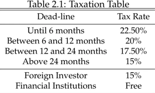
2.6 Taxes and Transactions Fees
As a matter of taxation, the lender income is treated as a fixed income and is taxed in accor-dance to Table 2.1:
6More information is available in the BM&FBovespa web site: http://www.bmfbovespa.com.br/
garantias/garantias.aspx?Idioma=en-us
Table 2.1: Taxation Table
Dead-line Tax Rate
Until 6 months 22.50%
Between 6 and 12 months 20%
Between 12 and 24 months 17.50%
Above 24 months 15%
Foreign Investor 15%
Financial Institutions Free
Typically a loan contract lasts at most 30 days and is qualified in the first line of Table 2.1. If income tax is applicable, it is discounted before exchange distributes payments.
BM&FBovespa charges borrowers inventors transaction fee of 0.25% over the contract finan-cial volume, respecting the mininal of minimal of R$10 per contract. In the case of automatic loan contracts the charge is 0.50%.
2.7 Automatic Loan
Chapter 3
Database Description
The Brazilian framework configures a unique opportunity to academic research on securi-ties lending and short selling. Due to the fact that market is centralized by BM&FBovespa, the stock exchange keeps records for the complete market in all stages of trade. BM&FBovespa treats a loan transaction as a process of three different stages: offers, contracts and liquidation. The data of each stage is recorded in three relational data bases in a way that the whole loan transaction process can be tracked. We have collected data from from these three databases for the period that goes from January 2007 to June 2013, the only masked fields are those contain-ing confidential information, like investor ID number and the offer’s directional field 1 . We
dedicate this section to describe in detail the data set we used to perform our analyzes.
3.1 Offers Database
All offers posted in the BTC platform, lending or borrowing, are recorded in the offers database. For some securities most offers are public and the recorded lending offers represent
the loan supply. Moreover, there are securities for which most of the offers are directional and dealers use the platform just for registration. We also can distinguish the type of final investor (as he is registered in the exchange) who posts the offer. Summarizing, in offers data set we have fields indicating:
• Date when offer was posted;
• Type of offer: borrower or lender;
• Name and number of securities;
• Index discriminating of which price should be considered in the liquidation (VWAP of the day before contract of before liquidation);
• Lending fee and broker’s commission rates;
• Index discriminating if the lender maintains his right of recall;
• Type of final investor: Individual person, mutual funds, commercial banks, investment banks, pension funds, foreign investors, etc.
1When a offer is directional, the directional field contains the broker’s ID to whom that offer was posted. This is
3.2 Contracts Database
Contracts databaserecords all loan contracts. A contract originates from two previously
reg-istered offers: lender offer and borrower offer. When there is demand in the market for a loan, the contract is settled as soon as BM&fbovespa recognizes the deposit of required collateral deposit, when it happens the contract is actually validated and registered. In the contracts database we have the following fields:
• Opening date;
• Offers numbers;
• Lending fee and commissions rates;
• Type of contract: lender, borrower, renovation, automatic, originated by dividends, etc;
• Name and number of securities;
• Brokers;
• Type of final investors.
3.3 Liquidation Database
Shares devolution may occur in multiple installments. Each (partial) devolution generates a liquidation event that is registered in theliquidation database. Each liquidation event refers to
the originating contract through the "Contract Number" field.
• Solicitation date,
• Maturity;
• Name and number of securities liquidated;
• Value debited/credited in each player account;
• Security price;
• Duration, in business days, of the contract.
3.4 Complementary Databases
Chapter 4
Empirical Facts about the Loan Market
In this chapter, we present the empirical findings of this thesis. In section 4.1 we introduce the key metrics we use to perform our analysis and an analysis of the market growth, shares among players and average loan fee behavior along time. Section 4.2 and 4.3 analyze how the loan fee depends on stock characteristics and what are the main differences among differ-ent types of market participants. We conclude our analysis by presdiffer-enting, in section 4.4, the summary statistics on contracts with right to recall in contrast to which without right of recall.
4.1 Volume, Players and Fees
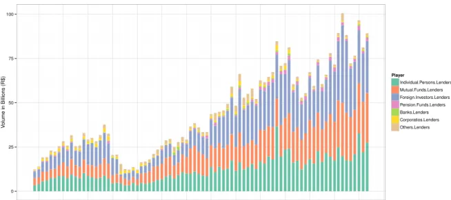
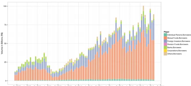
The aim of this section is to present an overview of the evolution of the Brazilian lending market between 2007 and 2013. We may resume the data presented in this section by saying that, between 2007 and 2013, the Brazilian lending market on average experienced an annual volume growth of 23.5%, and a loan fee decrease of 43 basis points. Approximately 90% of the lenders is equally composed by retail investors, domestic mutual funds or foreign investors, while borrowers are composed mainly by domestic mutual funds (56.7%) and foreign investors (27,8%).
In order to describe the market, we introduce three variables: the loan balance, the relative balance and the loan fee. The four variables are computed by aggregating, for each stock and each trading day, the transaction data contained in the trades database described in Subsection 3.2.
We define theloan balanceas the total number of shares borrowed in a single day multiplied
by the daily VWAP of the stock. Therelative balanceis given by loan balance over daily traded
volume, this is a measure of the impact that borrowed shares could have in the market. The (average)loan feeis the volume weighted average fee, calculated as:
Loan Feei,t = Ni,t X n=1
Loan Amountn,i,t PNi,t
n=1Loan Amountn,i,t
·Loan Feen,i,t !
(4.1)
whereNi,tis the number of transaction occurred for stockiin dayt, while Loan Feen,i,tand
Loan Amountn,i,t are the lending fee and borrowed amount of shares of the n-th individual
transaction.
90% of the total volume, and their share are roughly equally balanced. Figure 4.2 represents the same quantity, divided by type of borrower. For borrowers, the main types of players are just domestic mutual funds and foreign investors. Retail investors on average account for less then 4% of the total borrowed volume in the BTC market, while mutual funds accounts for 56.7% and foreign investors for 27.8%1.
Table 4.1 shows the participation in Bovespa’s segment, we are interested in comparing players’ shares in the BTC market to those in the equity market2. Although players’
character-ization are different between the two data sets, we conclude that retail person, institutional in-vestor (includes mutual funds) and foreign inin-vestors are also responsible for majority of trades in the equity market, as in the BTC market.
In the analyzed period the loan total balance had an average annual growth of 23.5%, de-spite the impact of the financial crises in 2008. In 2013, loan balance achieved two consecutive records: the first one in March, and the second in April, when it passed the landmark of R$100 billions.
0 25 50 75 100
Feb2007 Aug2007 Feb2008 Aug2008 Feb2009 Aug2009 Feb2010 Aug2010 Feb2011 Aug2011 Feb2012 Aug2012 Feb2013 Aug2013 Feb2014 Date
V
olume in Billions (R$)
Player
Individual.Persons.Lenders Mutual.Funds.Lenders Foreign.Investors.Lenders Pension.Funds.Lenders Banks.Lenders Corporatios.Lenders Others.Lenders
Figure 4.1: Loan Balance: Lenders
1Figures 4.1 and 4.2 were built using data available at http://www.bmfbovespa.com.br/
BancoTitulosBTC/Estatisticas.aspx?Idioma=en-us
0 25 50 75 100
Feb2007 Aug2007 Feb2008 Aug2008 Feb2009 Aug2009 Feb2010 Aug2010 Feb2011 Aug2011 Feb2012 Aug2012 Feb2013 Aug2013 Feb2014
V
olume in Billions (R$)
Player
Individual.Persons.Borrowers Mutual.Funds.Borrowers Foreign.Investors.Borrowers Pension.Funds.Borrowers Banks.Borrowers Corporations.Borrowers Others.Borrowers
Figure 4.2: Loan Balance: Borrowers
Table 4.1: Shares in Equity Market
Year Retail Investor Institutional Investors Foreign Investors Private and Public Companies Financial Institutions Others
2007 23.00% 29.80% 34.50% 2.20% 10.40% 0.20%
2008 26.84% 27.07% 35.33% 2.85% 7.81% 0.11%
2009 30.54% 25.67% 34.18% 2.15% 7.40% 0.06%
2010 26.41% 33.29% 29.57% 2.31% 8.35% 0.06%
2011 21.69% 33.49% 34.79% 1.34% 8.61% 0.09%
2012 17.92% 32.09% 40.36% 1.51% 8.09% 0.04%
2013 15.46% 32.93% 42.67% 0.91% 7.99% 0.04%
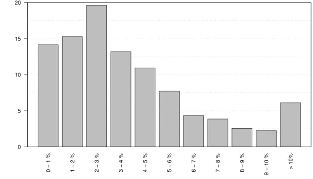
The histogram presented in Figure 4.3 represents the distribution of the annual average loan fees for each stock between January 2007 and June 2013. The vertical axis shows the frequency of firms with average loan fees in the interval displayed in the horizontal axis. The figure shows that 87.82% of the Brazilian market is on average special3. To have a better look, some of the
distribution quantiles are reported in Table 4.2.
0 − 1 % 1 − 2 % 2 − 3 % 3 − 4 % 4 − 5 % 5 − 6 % 6 − 7 % 7 − 8 % 8 − 9 %
9 − 10 %
> 10%
0 5 10 15 20
Loan Fee Average
Frequency (%)
Figure 4.3: Distribution of Loan Fees By Firms: 2007-2013
Table 4.2: Fee Distribution by Firms
Quantile Fee Average
10% 0.870
25% 2.120
50% 3.550
75% 5.500
90% 8.090
Along with the loan balance increase, one can observe significant reduction in the loan fee for some securities, what makes the fee distribution represented above more left skewed through time.
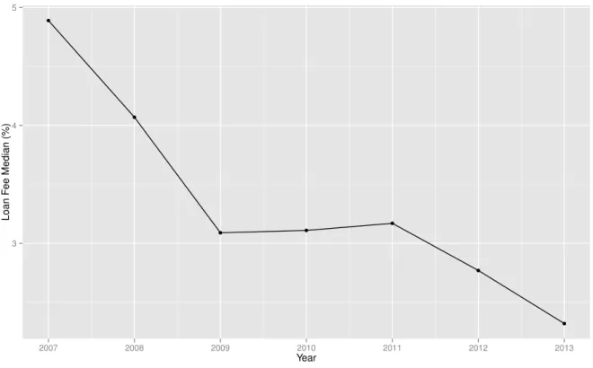
The graph in Figure 4.4 shows the fee distribution calculated in essentially the same way as in the graph reported in Figure 4.3 but on a yearly basis. In this graph, a tendency of the loan fee to reduce in time can be observed. In order to elucidate this fact, Figure 4.5 shows the evolution of the median fee through time4.
4Since we wanted to preserve all observations in the sample, we preferred the median over the mean for its
0 − 1 % 1 − 2 % 2 − 3 % 3 − 4 % 4 − 5 % 5 − 6 % 6 − 7 % 7 − 8 % 8 − 9 %
9 − 10 %
> 10%
x2007 x2008 x2009 x2010 x2011 x2012 x2013
0 5 10 15 20 25
Loan Fee Average
Frequency (%)
Figure 4.4: Distribution of Loan Fees By Firms by Year
●
●
● ●
●
●
●
3 4 5
2007 2008 2009 2010 2011 2012 2013
Year
Loan F
ee Median (%)
4.2 Fee Dependence
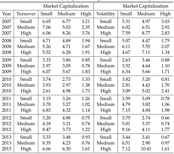
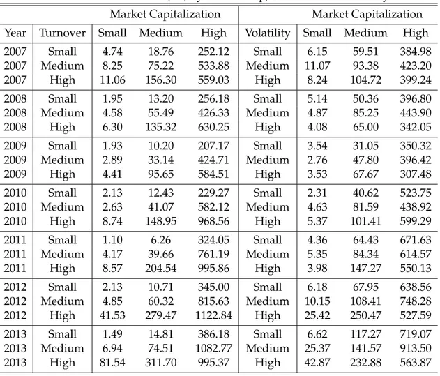
In this section we explore the the correlation of loan fee and loan balance with securities’ turnover, return volatility and market capitalization. The methodology I adopt is inspired by the one presented in D’Avolio (2002). The motivation for this exercise is first to understand how securities characteristics affect the loan fee formation. Our finding are that loan fee and loan balance are increasing on turnover and volatility, loan balance is increasing on market capitalization and loan fee is decreasing. The results provide empirical evidence in support of the theoretical benchmark introduced by Miller (1977) that short selling restriction would be increasing on divergence of opinion.
Tables 4.3 and 4.4 provide a series of two-way sorts of the loan contracts. The methodology to generate those tables goes as follows: each month to every stock in the loan database with more than five business days observations is assigned a size ranking: small (market equity deciles 1, 2, and 3), medium (deciles 4, 5, 6,and 7)and large (deciles 8, 9, and 10), and rank-ings small, medium and high (respecting the same quartiles) also for turnover and volatility. Like this we are able to accommodate time depending rotations on stocks characteristic and increases samples size for each quadrant.
For the securities in each quadrant we compute the average among monthly loan fee and monthly loan balance. Monthly loan fee is the average loan fee in a month and monthly loan balance the sum of loan balance in the specific month.
I use data on price, trade volume and outstanding from Economatica’s database. The mea-sure of turnover for each stock is the average daily turnover calculated using data on daily transaction volume over the stock’s outstanding. The price volatility is calculated as the stan-dard deviation of log return stock in one month, we calculated the returns usingadjusted price
time series, which adjusts the time series for dividends and splits events, this avoids spurious volatility. Market capitalization was calculated as an average of the product of outstanding and average daily price.
One of the findings of this thisis is the influence of distribution of interest on capital (one form of dividends distribution on Brazil) over the loan fee and demand to loans. A better analysis of this event is present in the next section. In order to prevent from loan fee and loan balance distortions caused by this events we did not consider trades 2 weeks before or 1 week after the interest on capital distribution events.
Table 4.3: Loan Fee (%) by Market Cap, Turnover and Volatility
Market Capitalization Market Capitalization
Year Turnover Small Medium High Volatility Small Medium High
2007 Small 6.65 6.77 3.21 Small 5.31 4.97 3.03
2007 Medium 7.06 5.03 2.35 Medium 6.02 6.51 2.92
2007 High 6.06 8.26 3.76 High 7.59 8.77 2.83
2008 Small 4.71 4.89 1.94 Small 5.07 4.47 1.75
2008 Medium 5.26 4.71 1.67 Medium 6.11 5.55 2.07
2008 High 5.52 6.28 1.91 High 4.67 7.11 1.34
2009 Small 3.33 3.86 0.85 Small 2.63 3.46 0.88
2009 Medium 2.97 3.05 0.78 Medium 3.52 4.64 1.10
2009 High 6.07 5.67 1.83 High 6.34 5.66 1.71
2010 Small 3.74 2.73 1.33 Small 3.82 3.20 0.81
2010 Medium 3.93 2.97 1.38 Medium 2.81 4.43 1.70
2010 High 2.61 4.98 1.73 High 3.09 5.02 2.41
2011 Small 3.15 3.26 1.26 Small 3.59 3.09 0.78
2011 Medium 3.70 3.27 1.02 Medium 4.79 3.82 1.06
2011 High 6.83 4.32 1.14 High 7.15 4.84 1.98
2012 Small 3.20 4.88 0.75 Small 3.75 2.74 0.66
2012 Medium 4.18 3.21 0.74 Medium 5.01 3.37 0.74
2012 High 8.47 3.73 1.22 High 9.16 4.11 1.77
2013 Small 3.33 3.48 0.93 Small 3.44 3.41 0.67
2013 Medium 8.35 4.23 0.76 Medium 6.51 2.90 0.97
Table 4.4: Loan Balance (mi) by Market Cap, Turnover and Volatility
Market Capitalization Market Capitalization
Year Turnover Small Medium High Volatility Small Medium High
2007 Small 4.74 18.76 252.12 Small 6.15 59.51 384.98
2007 Medium 8.25 75.22 533.88 Medium 11.07 93.38 423.20
2007 High 11.06 156.30 559.03 High 8.24 104.72 399.24
2008 Small 1.95 13.20 256.18 Small 5.14 50.36 396.80
2008 Medium 4.58 55.49 426.33 Medium 4.87 85.25 443.90
2008 High 6.30 135.32 630.25 High 4.08 65.00 342.05
2009 Small 1.93 10.20 207.17 Small 3.54 31.05 350.32
2009 Medium 2.89 33.14 424.71 Medium 2.76 47.80 396.42
2009 High 4.41 95.65 584.51 High 3.53 67.67 307.48
2010 Small 2.13 12.43 229.27 Small 2.31 40.62 523.75
2010 Medium 2.63 41.07 582.12 Medium 4.63 81.59 438.92
2010 High 8.74 148.95 968.56 High 5.37 101.41 599.29
2011 Small 1.10 6.26 324.05 Small 4.36 64.43 671.63
2011 Medium 4.17 39.66 761.19 Medium 5.35 84.34 614.57
2011 High 8.57 204.54 995.86 High 3.98 147.27 550.13
2012 Small 2.13 10.71 345.00 Small 6.18 67.95 638.56
2012 Medium 4.85 60.32 815.63 Medium 10.15 108.41 748.28
2012 High 41.53 279.47 1122.84 High 25.42 250.47 527.59
2013 Small 1.49 14.81 386.18 Small 6.62 117.27 719.07
2013 Medium 6.94 74.51 1082.77 Medium 25.37 141.57 913.50
2013 High 81.54 311.70 995.37 High 42.87 232.88 563.87
Although there are some exceptions, in Table 4.3 we observe that loan fee is increasing with turnover and volatility and decreasing with market cap. On the other hand, in Table 4.4 we see that loan balance seems to increase with volatility and turnover and market cap.
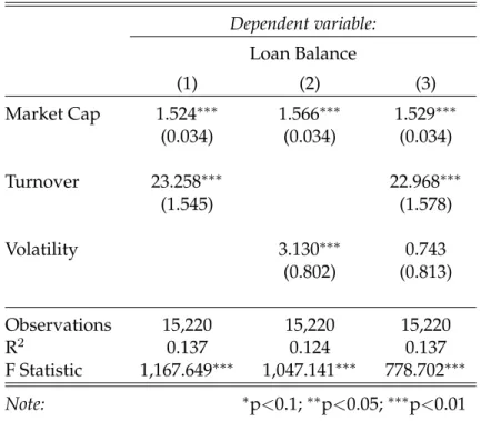
In order to have a more robust result about the correlation among this variables, I run two panel regressions, relating monthly data of loan fee and short interest to asset’s turnover, volatility and the of the market cap. I used fixed time effects of individual and time in other to account to heterogeneity among securities and through time, and I took the logarithmic of loan balance and market capitalization.
Table 4.5: Loan Fee Panel Regressions
Dependent variable:
Loan Fee
(1) (2) (3)
Market Cap −0.483∗∗∗ −0.267∗∗∗ −0.366∗∗∗
(0.073) (0.074) (0.073)
Turnover 62.122∗∗∗ 50.456∗∗∗
(3.285) (3.439)
Volatility 38.251∗∗∗ 26.988∗∗∗
(2.370) (2.471)
Observations 12,086 12,086 12,086
R2 0.032 0.024 0.042
F Statistic 194.995∗∗∗ 146.285∗∗∗ 171.067∗∗∗
Note: ∗p<0.1;∗∗p<0.05;∗∗∗p<0.01
Table 4.6: Loan Balance Panel Regressions
Dependent variable:
Loan Balance
(1) (2) (3)
Market Cap 1.524∗∗∗ 1.566∗∗∗ 1.529∗∗∗
(0.034) (0.034) (0.034)
Turnover 23.258∗∗∗ 22.968∗∗∗
(1.545) (1.578)
Volatility 3.130∗∗∗ 0.743
(0.802) (0.813)
Observations 15,220 15,220 15,220
R2 0.137 0.124 0.137
F Statistic 1,167.649∗∗∗ 1,047.141∗∗∗ 778.702∗∗∗
Note: ∗p<0.1;∗∗p<0.05;∗∗∗p<0.01
fees (represented by the aggregate loan fee). The effect should be the other way around when considering market capitalization. In this case the loan fees should decrease with market cap, since assets with grater float should be the ones with less asymmetric information (easier ac-cess to information) and also, their greater volume reduces the probability that non-lenders could hold relevant amount of shares what would pressure loan fees. If we assume that market capitalization, turnover and volatility reveal information about market disagreement, then our results are aligned with those of D’Avolio.
4.3 Players Analysis
One important concern of this research is to analyze traders’ accessibility to the loan market, and also investigate the presence of informed traders. Our first approach was to understand the differences in the loan fees in borrowers and lenders contracts among different players. We concentrate our analyzes on the most three representative players in accordance with loan balance. As presented before those players are: individual persons, domestic mutual fund and foreign investors. Although further analyzes are necessary to fully understand the role of each player in the market, our analysis suggests that different players have different conditions to participate in the lending market, what generates distortions on loan fee payed/charged among different players. For instance, retail investor and foreign investors pay larger loan fee to borrow securities when compared to mutual fund. The relationship is the other way around when we analyze the loan fee received for lending securities, mutual funds are able to charge larger fees when compared to retail investor and foreign investors.
In order to distinguish loan fees among player we now consider loan aggregation in stock, day and player. Loan fee for playerpis calculated as below:
Loan Feei,t,p = Ni,t,p
X n=1
Loan Volumen,i,t,p PNi,t,p
n=1 Loan Volumen,i,t,p
·Loan Feen,i,t,p !
(4.2)
where n denotes the transaction, i stands for securities, t the day in which the contract is opened, p the player type andNi,t,p is the total number of contracts for security i in the day t
for player p.
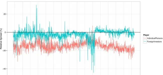
Figures 4.6 and 4.7 shows the evolution of relative spread of loan fees payed and received by individual person and foreign investors when compered to mutual funds5 6. Relative spread
is calculated as:
Relative Spreadi,t,p = Loan Feei,t,p−Loan Feei,t,fund
Loan Feei,t,fund (4.3)
5We just consider dates and stocks where there are trades from the three players considered
6An aggregate result may take to a misleading result, but we did this exercise to selected securities separately
−40 −20 0 20
Feb2007 Jul2007 Dec2007 May2008 Oct2008 Mar2009 Aug2009 Jan2010 Jun2010 Nov2010 Apr2011 Sep2011 Feb2012 Jul2012 Dec2012 May2013 Oct2013
Relativ
e Spread (%)
Player
IndividualPersons
ForeignInvestors
Figure 4.6: Mutual Funds Fee Relative Spread: Lender
0 50 100 150
Feb2007 Jul2007 Dec2007 May2008 Oct2008 Mar2009 Aug2009 Jan2010 Jun2010 Nov2010 Apr2011 Sep2011 Feb2012 Jul2012 Dec2012 May2013 Oct2013
Relativ
e Spread (%)
Player
IndividualPersons ForeignInvestors
Figure 4.7: Mutual Funds Fee Relative Spread: Borrower
4.4 Right of Recall
A loan contract can guarantee the lender theright of recall, i.e. the right to force the closing
of the contract, and hence the devolution of the borrowed stocks, before the contract maturity. This type of loan contracts carry an additional risk for the short seller, who may be forced to close his position, or engage in another contract with a higher fee. For this reason, this type of contracts should be treated differently from the others.
Contracts with right of recall were implemented in Brazil in 2011, and quickly gained pop-ularity among market participants. Table 4.4 shows the percentage of contracts with right of recall over all contracts. The use of contracts with right of recall is in accordance with the standard practice in the US markets, where they are the most common type of contracts.
Table 4.7: Presence of Recall Right
Year Recall No-Recall
2011 0.34% 99.66%
2012 24.59% 75.41%
2013 45.77% 54.23%
In order to determine how the risk of recall is priced in the loan fee, we selected the stocks for which both type of contracts are available, and computed the respective average loan fee for the period 2012-2013. As expected, the average loan fee of contracts with right of recall turned out to be lower, the difference between the two averages being of0.47%.
To examine the variability of this spread among individual securities, we compute the two average loan fees over the same period for the main securities analyzed in??. Table 4.8 shows that contracts with right of recall always have a higher average loan fee, and that the spread can vary from 0.01% up to 1.4%. By looking at Table 4.9, we deduce that, at the individual stock level, no clear asymmetry pattern seems to be present in the frequency of one type of contract or the other.
Table 4.8: Important Securities: Average Fee (%)
CODE No-Recall Recall
AMBV3 0.353 0.239
AMBV4 0.236 0.226
PETR3 0.713 0.399
PETR4 2.202 0.777
VALE3 0.603 0.509
Table 4.9: Important Securities - Number of Contracts (millions)
CODE No-Recall Recall
AMBV3 25.10 16.55
AMBV4 25.57 16.71
PETR3 59.51 85.22
PETR4 64.05 108.50
VALE3 39.61 52.45
Chapter 5
Tax Arbitrage
In this chapter we perform individual stocks analysis that unveil an stylized fact about the Brazilian lending market, a tax arbitrage opportunity. When considering the loan fee time se-ries of individual stocks we were able to identify large fluctuations on loan fee and relate those events to one type of dividends distribution specific of the Brazilian market called: interest on net equity (IoNE). Brazilian hedge funds have favorable tax legislation when compared to other agents, this fact generates a tax arbitrage opportunity. Although it is a known fact by financial market professionals, it was never studied in detailed in an academic framework.
The analyzed securities were chosen according to criteria of liquidity and stability: they are among those with higher loan balance and, in the analyzed period, they did not go through major institutional changes. We selected VALE5 (12.5% of the total balance considering), PETR4 (7.5% of the total balance) and AMBV4 (3.7% of the total balance)1. We add to this list OGXP3
due to recent events specific to this stock that were relevant to the lending market.
For each stock we plot five graphs representing the evolution in time of the main statistics of the lending market. The first graph shows the evolution in time of stock’s VWAP2, the second
shows the evolution of the loan fee, third graph shows relative balance, fourth number of lent stocks and fifth our measure of short interest.
A clear pattern emerging from Figures 5.1, 5.2 and 5.3 is the presence of spikes in loan fee and quantity time series. For PETR4 for example, the loan fee jumps to 31.59%, although its historical loan fee average is 0.62%. A similar phenomenon is observed with VALE5, where the loan fee jumps to 26.61%, while its historical loan fee average is 0.53%. The origin of these spikes will be discussed in the next subsection.
The relative balance evolution also has some abnormal features. Anaive thinking would
suggest that relative balance would be a reasonable proxy of traded volume originated by bor-rowed securities, however, a closer look at the data shows that this value can go beyond 400% for PETR4, for example, or 2000% for AMBV4. This is a clear signal that not all the borrowers are actually interested in selling the asset. Different hypothesizes can to explain this type of event: hedging strategies, in special hedging of call options, dividends distribution, etc.
1We did not analyze ITUB4 because of the merger of Itau with Unibanco in 2009.
20 25 30 35 40 45
2007 2008 2009 2010 2011 2012 2013
Pr
ice
Price
0 10 20
2007 2008 2009 2010 2011 2012 2013
Loan F
ee(%)
Loan Fee
0 1 2 3 4
2007 2008 2009 2010 2011 2012 2013
Relativ
e Balance
Relative Balance
0 20 40 60
2007 2008 2009 2010 2011 2012 2013
Millions
Number of Stocks
0.0 0.5 1.0 1.5
2007 2008 2009 2010 2011 2012 2013
Shor
t Interest(%)
Short Interest
20 30 40
2007 2008 2009 2010 2011 2012 2013
Pr
ice
Price
0 10 20 30
2007 2008 2009 2010 2011 2012 2013
Loan F
ee(%)
Loan Fee
0 1 2 3 4
2007 2008 2009 2010 2011 2012 2013
Relativ
e Balance
Relative Balance
0 50 100
2007 2008 2009 2010 2011 2012 2013
Millions
Number of Stocks
0.00 0.25 0.50 0.75 1.00
2007 2008 2009 2010 2011 2012 2013
Shor
t Interest(%)
Short Interest
25 50 75
2007 2008 2009 2010 2011 2012 2013
Pr
ice
Price
0 1 2 3 4
2007 2008 2009 2010 2011 2012 2013
Loan F
ee(%)
Loan Fee
0 5 10 15 20
2007 2008 2009 2010 2011 2012 2013
Relativ
e Balance
Relative Balance
0 25 50 75 100 125
2007 2008 2009 2010 2011 2012 2013
Millions
Number of Stocks
0.0 0.2 0.4 0.6
2007 2008 2009 2010 2011 2012 2013
Shor
t Interest(%)
Short Interest
0 5 10 15 20
2009 2010 2011 2012 2013
Pr
ice
Price
0 10 20 30 40 50
2009 2010 2011 2012 2013
Loan F
ee(%)
Loan Fee
0 10 20 30
2009 2010 2011 2012 2013
Relativ
e Balance
Relative Balance
0 20 40 60
2009 2010 2011 2012 2013
Millions
Number of Stocks
0.0 0.5 1.0 1.5 2.0
2009 2010 2011 2012 2013
Shor
t Interest(%)
Short Interest
Figure 5.4: Time Series: OGXP3
arbitrage consists in changes in stock ownership around dividends payment to investor that are domiciled in the country with favorable divided tax legislation. The impact of tax arbitrage in a world-wide perceptive is commented in Saffi and Sigurdsson (2011). This phenomenon can have significative impact in the lending market and a credible empirical work has to account these deviations.
To understand the Brazilian case, first it is necessary to overview the tax legislation. Brazil-ian companies have two main instruments for remunerating shareholders for the capital invested in companies: dividends and interest on net equity (“Juros sobre o capital própio”) -IoNE. Both instruments can be used at the same time, but their tax treatment will depend on the particular characteristics of each case. While dividends feature exists in most jurisdictions, IoNE is unique to the Brazilian system.
Distribution of IoNE paid to Brazilian and non-Brazilian holders of preferred shares, includ-ing payments to the Depositary in respect of preferred shares underlyinclud-ing ADSs, are deductible by TNL for Brazilian corporate income tax purposes. Such payments are subject to Brazilian withholding tax at the income tax rate of 15%, except for payments to persons who are exempt from income tax in Brazil, which payments are free of income tax, and except for payments to persons situated in tax havens, which payments are subject to an income tax at a 25% rate. All taxes are charged in source, even if recipient is nonresident 3. On the other hand, dividends
are not deductible by TNL but when received by shareholders there are no additional income taxes.
In the Brazilian regulation there is an upper limit on IoNE is determined as the higher of 50% of net income for the year. This taxation method is justified by Brazilian policy makers as an incentive to companies increase their capitalization.
Although dividends payments seem to have no impact on loan fees, Figures 5.5, 5.6 and 5.7 show that IoNE matches exactly to the spikes found in the last subsection.
0 1 2 3 4
2007 2008 2009 2010 2011 2012 2013
Lending F
ee(%)
Lending Rate Evolution
Figure 5.5: IoNE Settlement Date: AMBV4
0 10 20
2007 2008 2009 2010 2011 2012 2013
Lending F
ee(%)
Lending Rate Evolution
Figure 5.6: IoNE Settlement Date: VALE5
0 10 20 30
2007 2008 2009 2010 2011 2012 2013
Lending F
ee(%)
Lending Rate Evolution
Figure 5.7: IoNE Settlement Date: PETR4
the financial volume of the IoNE) minus the financial volume payed to loan contract.
All stocks that pay IoNE are subject to tax arbitrage. The mechanism through what gains are shared among players is an increase in loan fees. In Figure 5.8 we selected the stocks that presented IoNE events during the analyzed period in order to observe the behavior of loan fees around the settlement date. The x-axis of this graph represents an average loan fees per day from settlement date, represented in the y-axis.
● ● ● ●
● ●
● ● ●●
●● ●
●● ●●
● ●
●● ●
● ●
● ●
● ●
● ●
●
● ●
● ●
● ●● ●
● ●
● ●
● ● ●●
● ●
● ●
● ●●
● ●
● ●
●● ●
3 4 5 6
−30 −25 −20 −15 −10 −5 0 5 10 15 20 25 30
Time Difference to IoNE actualization date (days)
A
ver
age Loan F
ee (%)
Figure 5.8: Lending Fee around IoNE Settlement date Date
In the graph of Figure 5.8 we observe that thirty days before IoNE settlement the average loan fee is 2.36% and increases to 6.11% on the settlement date. The increase is sharper in the three days before settlement date, that corresponds to the time difference between IoNE announcement and settlement.
5.1 Case Study: PETR4
In order to elucidate this practice we choose Petrobras’ IoNE distribution on May 3rd, 2013 as an example. On April 30th, 2013 Petrobras announced that would payR$0.76per share of PETR4. In Brazil, trades are liquidated in D+3, so the settlement date of this IoNE was May 3rd
4.
Each dot of Figure 5.9 represents a loan contract, the x-axis is the contract openness date and y-axis the loan fee agreed. The dotted line represents the settlement date. In this figure we observe that the closer the settlement date the higher the loan fees become. The loan growth is sharper between the announcement date (April 30th) and the settlement date, this is indeed expected, since there are no more uncertainties about the settlement date or value of the IoNE in this period.
4Settlement datecorresponds to date that the company computes and registers the income of each shareholder.