International competition and labor market adjustment

ISSN 2042-2695

CEP Discussion Paper No 1411

March 2016

International Competition and Labor Market Adjustment

Abstract

How does welfare change in the short- and long-run in high wage countries when integrating with low wage economies like China? Even if consumers benefit from lower prices, there can be significant welfare losses from increases in unemployment and lower wages. I construct a dynamic multi-sector-country Ricardian trade model that incorporates both search frictions and labor mobility frictions. I then structurally estimate this model using cross-country sector-level data and quantify both the potential losses to workers and benefits to consumers arising from China’s integration into the global economy. I find that overall welfare increases in northern economies, both in the transition period and in the new steady state equilibrium. In import competing sectors, however, workers bear a costly transition, experiencing lower wages and a rise in unemployment. I validate the micro implications of the model using employer-employee panel data.

Keywords: trade, unemployment, earnings, China JEL codes: F16; J62; J64

This paper was produced as part of the Centre’s Growth Programme. The Centre for Economic Performance is financed by the Economic and Social Research Council.

I am grateful to John Van Reenen, Gianmarco Ottaviano and Emanuel Ornelas for their guidance and support. I am also thankful to Alan Manning, Andy Feng, Catherine Thomas, Chris Pissarides, Claudia Steinwender, Cl\'ement Malgouyres, Daniel Junior, Daniela Scur, David Dorn, Francisco Costa, Frank Pisch, Jason Garred, John Morrow, Jonathan Colmer, Katalin Szemeredi, Markus Riegler, Mirko Draca, Oriol Carreras, Pedro Souza, Steve Machin, Steve Pischke, Stephen Redding, Tatiana Surovtseva, Thomas Sampson and seminar participants at LSE, EGIT Research Meeting, IAB Spatial LM Workshop, TADC, CEP Annual Conference, Erasmus University Rotterdam, Bocconi University, FED Board, UC Boulder, PUC-Rio, FGV-EESP, FGV-EPGE, INSPER, FEA-USP, SBE Meeting and RIDGE Workshop. All remaining errors are mine.

João Paulo Pessoa, FGV-Sao Paulo School of Economics and Associate at Centre for Economic Performance, London School of Economics.

Published by

Centre for Economic Performance

London School of Economics and Political Science Houghton Street

London WC2A 2AE

All rights reserved. No part of this publication may be reproduced, stored in a retrieval system or transmitted in any form or by any means without the prior permission in writing of the publisher nor be issued to the public or circulated in any form other than that in which it is published.

Requests for permission to reproduce any article or part of the Working Paper should be sent to the editor at the above address.

1

Introduction

It has been recognized that trade openness is likely to be welfare improving in the

long-run, by decreasing prices and allowing countries to expand their production to new

mar-kets. These gains, however, generally neglect important labor market aspects that take

place during the adjustment process, such as displacement of workers in sectors harmed

by import competition and the fact that workers do not move immediately to growing

exporting sectors.

In the last decades China has emerged as powerful player in international trade. In

2013, it surpassed the United States (US) to become the world’s largest goods trader in

value terms. In this paper I study how countries adjust to the rise of China in a world

with imperfect labor markets.

The main contribution of this paper is to provide a tractable framework to structurally

quantify the impact of trade shocks in a world with both search frictions and labor

mo-bility frictions between sectors. I calculate changes in real income per capita arising

from the emergence of China using numerical methods, both in the new equilibrium and

along the transition period. My calculations take into account not only the benefits but

also account for potential costs linked to labor market adjustments. I find that China’s

integration generate gains worldwide also in the short-run. However, there are winners

and losers in the labor market.

My dynamic trade model incorporates search and matching frictions fromPissarides

(2000) into a multi-country-sector Costinot, Donaldson, and Komunjer (2012) frame-work.1 In this set-up goods can be purchased at home, but consumers will pay the least-cost around the world accounting for trade least-costs. Hence, individuals benefit from more

trade integration by accessing imported goods at lower costs. On the other hand, a rise in

import competition in a sector will decrease nominal wages and increase job destruction

in this sector. Wages will not be equal across sectors within countries because of labor

mobility frictions, which are added to the model assuming that workers have exogenous

preferences over sectors. To analyze how all these effects interact following a trade shock

I use numerical simulations.

The “China shock” used in my numerical exercise consists of a decrease in Chinese

trade barriers and an increase in Chinese productivity that emulates the growth rate of

China’s share of world exports following China’s entry to the WTO. I find that northern

economies gain from this shock. For example, annual real consumption in the US and

in the United Kingdom (UK) increase by 1.3% and 2.3%, respectively, in the new steady

state compared to the initial one.

The effects of the shock on wages and unemployment are heterogeneous across

sec-tors within countries. In low-tech manufacturing industries in the UK and in the US,

which face severe import competition from China, workers’ real wages fall and

unem-ployment rises. The fall in the real average wage in this sector is approximately 1.6%

in the US and 0.7% in the UK during the adjustment period five years after the shock.

However, at the same point in time workers in the service sector experience a rise in the

real average wage and no significant change in the unemployment rate: The real average

wage in services increases by approximately 1.9% in the US and 2.5% in the UK.

The numerical exercise also demonstrates the dynamic effects associated with the rise

of China. Immediately after the shock, nominal wages rise in exporting sectors and fall

in industries facing fierce import competition from China. As workers move from sectors

hit badly by China in search of better paid jobs in other industries, wages in exporting

sectors start to fall due to a rise in labor supply. This implies that wages are lower in the

final steady state than during the transition in these industries. In some import competing

sectors, however, the effects go in the opposite direction: Wages fall immediately after

the shock and recover over time.2

In order to perform counterfactual analysis I estimate a sub-set of the parameters of

the model using country-sector level data. I estimate a gravity equation delivered by the

model using data on bilateral trade flows to obtain the trade elasticity parameter. I also

use equations from my theoretical framework to estimate the parameters related to job

destruction and labor mobility frictions between sectors. The remaining parameters are

either calibrated or taken from the literature.

Even though countries experience overall real income gains in my counterfactual

exercise, workers in import competing sectors lose from a fall in real wages and an

in-crease in unemployment not only during the transition but also in the new steady state.

Another prediction from my model is that low-paid (low-productivity) jobs are the ones

2_{More precisely, in the low-tech manufacturing sector, wages fall during the first five years after the}

destroyed in sectors that experience a negative shock. I validate the qualitative

predic-tions discussed above by drawing on detailed employer-employee panel data from one

developed mid-size economy, the UK. Quantitative trade exercises usually focus on the

US. I also look at the US in my counterfactuals, but as a very large and rich country, I

find it useful to validate the micro implications of my model on a smaller and more open

economy, the UK.

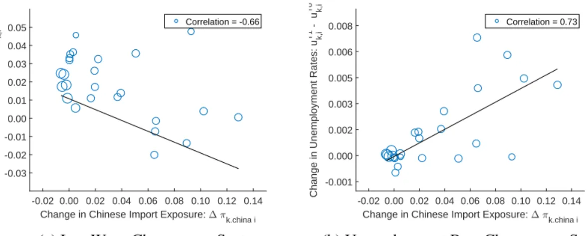
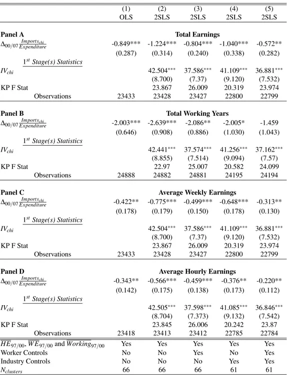
By analyzing the period between 2000 (the year before China entered into the WTO)

and 2007 (the year before the “Great Recession”) I provide support for the three main

predictions discussed, i.e., that more Chinese import competition in an industry: i)

de-crease worker’s earnings; ii) inde-crease worker’s number of years spent out of employment;

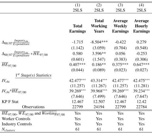
iii) has a stronger impact on low-paid workers.3

I find that workers initially employed in industries that suffered from high levels

of import exposure to Chinese products between 2000 and 2007 earned less and spent

more time out of employment when compared to individuals that were in industries less

affected by imports from China. I find a negative and significant effects in terms of both

weekly and hourly earnings, and that workers that received lower wages between 1997

and 2000 (a proxy for skills) experienced higher subsequent employment losses between

2000 and 2007.

Many other papers study the effects of trade openness on labor markets by

quantify-ing theoretical models. However, to my knowledge this is the first paper that explicitly

quantifies the effects of a trade shock, the emergence of China, analyzing all the

follow-ing aspects: general equilibrium effects across countries, the dynamic adjustment path

to a new equilibrium (in a set-up where jobs can be endogenously destroyed) and labor

mobility frictions between sectors.4

3_{My empirical strategy builds onAutor, Dorn, Hanson, and Song(2014).}

4_{Caliendo, Dvorkin, and Parro(2015) develop a dynamic trade model with full employment that takes} into account labor mobility frictions, goods mobility frictions, geographic factors and input-output link-ages. They calibrate the model to 22 sectors, 38 countries and 50 states in the US to quantify the effects of the China shock. They find that China was responsible for the destruction of thousands of jobs in manu-facturing in the US, but the shock generated aggregate welfare gains.di Giovanni, Levchenko, and Zhang

An example of a paper that quantifies the effects of a trade shock on labor markets

isArtuc, Chaudhuri, and McLaren(2010), where the authors consider a dynamic model with labor mobility frictions across sectors. They estimate the variance of US workers’

industry switching costs using gross flows across industries and simulate a trade

liber-alization shock. This and other papers in this literature, however, consider a small open

economy set-up, disregarding general equilibrium effects across countries.5

Another strand of the literature quantifies models in which labor markets are

imper-fect taking into account general equilibrium efimper-fects across countries, but usually ignore

multi-sector economies (and consequently that workers do not move freely between

sec-tors) and are silent about transitional dynamics, due to the static nature of their

frame-work. The most similar paper to mine in this area isHeid and Larch (2012), that con-siders search generated unemployment in anArkolakis, Costinot, and Rodriguez-Clare

(2012) environment and calculate international trade welfare effects in the absence of full employment.6

The validation of the predictions of my model also contributes to the literature that

uses worker level information to identify effects of international trade on labor market

outcomes, including out of employment dynamics. Examples areAutor, Dorn, Hanson, and Song(2014), which considers the China shock to identify impacts on labor markets in the US, andPfaffermayr, Egger, and Weber(2007), which uses Austrian data to esti-mate how trade and outsourcing affect transition probabilities between sectors and/or out

5_{Another interesting paper isDix-Carneiro(2014), which estimates a dynamic model using Brazilian} micro-data to study the adjustment path after a Brazilian trade liberalization episode in the nineties. Utar

(2011) calibrates a model using Brazilian data to answer a similar question, whileHelpman, Itskhoki, Muendler, and Redding(2012) use linked employer-employee data to analyze also the trade effects in this same country, but with a greater focus on wage inequality. Cosar, Guner, and Tybout (2013) andUtar

(2006) use Colombian firm level data to estimate a dynamic model of labor adjustment and study how the economy fairs following an import competition shock. Kambourov(2009) builds a dynamic general equilibrium sectoral model of a small open economy with sector-specific human capital, firing costs and tariff. He calibrates the model using Chilean and Mexican data to quantify the effects of trade reforms that took place in the seventies and in the eighties in Chile and in Mexico, respectively, finding that if a country does not liberalize its labor market at the outset of its trade reform, the reallocation of workers across sectors will be slower, reducing the gains from trade.

6_{Felbermayr, Larch, and Lechthaler(2013) construct a static one sector Armington model with frictions} on the goods and labor markets and use a panel data of developed countries to verify the predictions of the model.Felbermayr, Impullitti, and Prat(2014) builds a dynamic two country one sector model a laMelitz

of employment states.7

The paper is organised as follows. In Section 2 I present my model and discuss its

most important implications. In section 3 I structurally estimate a sub-set of the

param-eters of the model, explain how to numerically compute my counterfactual exercise and

present its results. In Section 4 I validate the key micro implications of the model using

employer-employee panel data from the UK. I offer concluding comments in Section 5.

2

Model

My dynamic trade model incorporates frictional unemployment with endogenous job

destruction (Pissarides,2000) into a multi-country/multi-sectorCostinot, Donaldson, and Komunjer(2012) framework. I also add labor mobility frictions between sectors using some features fromArtuc, Chaudhuri, and McLaren(2010).

The model takes into account that labor markets are imperfect. The economy is

composed of many countries and sectors. Workers without a job can choose the sector

in which to search for employment according to their personal exogenous preferences.

Within a sector, firms and workers have to engage in a costly and uncoordinated process

to meet each other. Each sector produces many types of varieties, and consumers will

shop around and pay the best available price for each type of variety (considering trade

costs).

The model is tractable and allows the ability to quantify changes in real income per

capita (my welfare proxy) following a trade shock (the emergence of China)

consider-ing not only the positive aspects associated with cheaper consumption goods but also

the potential negative aspects associated with labor market adjustments. My dynamic

framework will also enable me to study how different groups of workers are affected

at different points in time. I start the section by providing the main components of the

model. I then demonstrate how to compute the equilibrium and discuss some of the

implications of the model.

7_{More broadly, the paper adds to a growing literature on the effects of trade shocks on labor markets,}

2.1

Set up

In terms of notation, at_k,i represents variable ‘a’ in sector kin countryiat timet. Some

variables represent a bilateral relationship between two countries. In this case, the

vari-able at_k,oi is related to exporter o and importer i in sector k. Finally, in other cases it

will be necessary to highlight that a variable depends on a worker, on a variety or on a

different productivity level. In such cases, at_k,i(l) means that the variable is related to

the workerl, at_k,i(j)is a variable associated with the variety jandat_k,i(x)is linked to

id-iosyncratic productivityx. For the sake of simplicity, I omit the variety index jwhenever

possible.

2.1.1 Consumers

There are N countries. Each country has an exogenous labor force Li and is formed

by K sectors containing an (endogenous) mass of workers Lt_i,k and an infinite mass of

potential entrant firms. I assume that heterogeneous family members in each country

pool their income, which is composed of unemployment benefits, labor income, firm

profits and government lump-sum transfers/taxes, and maximize an inner C.E.S, outer

Cobb-Douglas utility function subject to their income:8

Max

∑

t

∑

k

µ_k,i ε

lnR₀1(Ct

k,i(j))εd j

(1+r)t .

Wherek indexes sectors,ε= (σ−1)/σ, σ is the constant elasticity of substitution

(between varieties) andC_kt_,i(j)represents consumption of variety j. µk,i is countryi’s

share of expenditure on goods from sectork, and ∑_kµ_i,k =1. Note that consumers do

not save in this economy. The dynamic effects in the model arise from labor market

features, as shown below.

8_{Under the assumption of a “big household” with heterogeneous individuals (employed/unemployed in}

different sectors), and that households own some share of firms, household consumption equals its income

Consumptiont_i=Incomet_i=Wagest_i+Pro f itst_i+U nempBene f itst_i+T govt_i

2.1.2 Labor Markets

Each sector has a continuum of varieties j∈[0,1]. I treat a variety as an ex-ante different

labor market. I omit the variety index j from this point forward, but the reader should

keep in mind that the following expressions are country-sector-variety specific.

Firms and workers have to take part in a costly matching process to meet each other in

a given market. This process is governed by a matching functionm(ut

k,i,vtk,i). It denotes

the number of successful matches that occur at a point in time when the unemployment

rate is ut_k,i and the number of vacancies posted is vt_k,i (expressed as a fraction of the

labor force). As inPissarides(2000), I assume that the matching function is increasing in both arguments, concave and homogeneous of degree 1. Homogeneity implies that

labor market outcomes are invariant to the size of the labor force in the market. For

convenience, I work withθt

k,i=vtk,i/utk,i, a measure of labor market tightness.

So the probability that any vacancy is matched with an unemployed worker is given

by

m(ut k,i,vtk,i)

vt_k,i =q(θ

t k,i),

and the probability that an unemployed worker is matched with an open vacancy is

m(ut k,i,vtk,i)

ut_k,i =θ

t

k,iq(θkt,i).

Workers are free to move between markets to look for a job but not between sectors

as will become clearer later. Unemployed workers receive a constant unemployment

benefitbi. New entrant firms are also free to choose a market in which to post a vacancy

and are constrained to post a single vacancy. While the vacancy is open they have to pay

a per period cost equals toκ times the productivity of the firm.

Jobs have productivityzk,ix. xis a firm specific component, which changes over time

according to idiosyncratic shocks that arrive to jobs with probability ρ, changing the

productivity to a new valuex′, independent ofxand drawn from a distributionG(x)with

support[0,1]. zk,iis a component common to all firms within a variety, constant over time

and taken as given by the firm (I postpone its description until the end of this subsection).

Conditional on producing variety j, each firm can choose its technology level and profit

opened with productivityz(at maximumx).

After firms and workers meet, production starts in the subsequent period. Firms are

price takers and their revenue will be equal topt_k,izk,ix. During production periods, firms

pay a wagewt_k,i(x)to employees.

When jobs face any type of shock (including the idiosyncratic one), firms have the

op-tion of destroying it or continuing producop-tion. LetJ_kt_,i(x)be the value of a filled vacancy

for a firm. Then, production ceases whenJ_kt_,i(x)<0 and continues otherwise. So, job

destruction takes place whenxfalls below a reservation levelRt_k,i, whereJ_kt_,i(Rt_k,i) =0.

Defining the expected value of an open vacancy asV_kt_,i, I can write value functions that

govern firms’ behavior:

V_kt_,i=−κpt_k,izk,i+

1 1+r[q(θ

t

k,i)Jkt,+i1(1) + (1−q(θ t

k,i))Vkt,+i1]. (1)

J_kt_,i(x) =pt_k,izk,ix−wtk,i(x) +

1 1+r[ρ

1 Z

Rt+_k,i1

J_kt+_,i1(s)dG(s) + (1−ρ)J_kt+_,i1(x)]. (2)

The value of an open vacancy is equal to the per-period vacancy cost plus the future

value of the vacancy. The latter term is equal to the probability that the vacancy is filled,

q(θt

k,i), times the value of a filled vacancy next period,J t+1

k,i (1), plus the probability that

the vacancy is not filled multiplied by the value of an open vacancy in the future, all

discounted by 1+r.

I am implicitly assuming that firms are not credit constrained, even though some

papers, e.g. (Manova, 2008), argue that financial frictions matter in international trade. So, governments will lend money to firms (financed by lump-sum taxes on consumers)

as long as the value of posting a vacancy is greater or equal to zero. The value of a filled

job is given by the per period revenue minus the wage cost plus the expected discounted

value of the job in the future. The last term is equal to the probability that idiosyncratic

shocks arrive multiplied by the expected value of the job next period,ρ 1 R

Rt+_k,i1

Jt_k+_,i1(s)dG(s), plus the value that the job would have in the absence of a shock times the probability of

such event,(1−ρ)J_kt+_,i1(x).

U_kt_,iandW_kt_,i(x)are, respectively, the unemployment and the employment value for a

U_kt_,i=bi+

1 1+r[θ

t k,iq(θ

t k,i)W

t+1

k,i (1) + (1−θ t k,iq(θ

t k,i))U

t+1

k,i ]. (3)

W_kt_,i(x) =wt_k,i(x) + 1 1+r[ρ(

1 Z

Rt+_k,i1

W_kt_,+_i1(s)dG(s) +G(R_kt+_,i1)U_kt+_,i1) + (1−ρ)W_kt_,+_i1(x)]. (4)

The unemployment value is equal to the per period unemployment benefit plus the

discounted expected value of the job next period, given that workers get employed with

probabilityθ_kt_,iq(θ_kt_,i).

The value of a job for a worker is given by the per-period wage plus a continuation

value, which is composed by two terms. First, the worker could get the value that the job

would have in the absence of a shock,W_kt_,+_i1(x), a value that is realised with probability 1−ρ. If a shock arrives, with probabilityρG(Rt_k+_,i1)the shock will be sufficiently bad to drive the worker into unemployment and he/she obtains onlyU_kt+_,i1 next period. If after the shock productivity remains above the destruction threshold, then the worker gets on

averageρ 1 R

Rt+_k,i1

W_kt_,+_i1(s)dG(s).

Wages are determined by means of a Nash bargaining process, where employees have

exogenous bargaining power 0<β_k,i<1. Hence, the surplus that accrues to workers

must be equal to a fractionβk,iof the total surplus,

W_kt_,i(x)−U_kt_,i=β_k,i(J_kt_,i(x) +W_kt_,i(x)−U_kt_,i−V_kt_,i). (5)

2.1.3 Firm Entry and Worker Mobility within a Sector

Remember that workers and firms are free to look for jobs and to open vacancies across

varieties. Hence, at every point in time the unemployment value must be equal for all

varieties that are produced in equilibrium. Because markets are competitive, firms cannot

obtain rents from opening vacancies. This implies that the value of a vacancy will be

equal to zero in any market inside a country. These two conditions can be summarised

as follows,

U_kt_,i(j) =U_kt_,i(j′) (6)

where here I explicitly indicate that the unemployment value and the value of an open

vacancy are ex-ante market specific.

The fact that unemployment values are equalised across different varieties (condition

6) implies thatpt_k,iz_k,imust be equal across markets that produce in equilibrium. Suppose

that there are two varieties j and j′ with distinct values of pt_k,izk,i and without loss of

generality, assume that job market tightness is greater in market j, meaning that it is

easier for a worker to find a job there. In this case, pt_k,iz_k,i must be greater in market

j′, such that the lower probability of finding a job in this market is compensated by

higher wages. However, if this is the case, firms will only be willing to open vacancies

in market j, where they have a higher probability of finding a worker and can pay lower

wages. Hence, the only possible equilibrium is a symmetric one whereθ_kt_,iandpt_k,izk,iare

equalised across varieties inside a sector in a country. Hence, all varieties also have the

same labor market outcomesRt_k,iandut_k,i, as well as the same wage distribution. As will

be discussed below, the only variety dependent variable is the price (a sketch of proof is

presented inAppendix A -).

2.1.4 Worker Mobility between Sectors

Before looking for a job in a particular sector, an unemployed worker must choose a

sec-tor, and in contrast to the variety case, they do not move freely between sectors. I assume

that each worker has a (unobserved by the econometrician) preferenceνk(l)for each

sec-tor, invariant over time. I further assume that workers know all the information necessary

before taking their decision. Hence, the value of being unemployed in a particular sector

for a workerl, ˆU_kt_,i(l), is given by

ˆ

U_kt_,i(l) =U_kt_,i+ν_k(l).

A highν_k(l)relative toν_k′(l)means that the worker has some advantage of looking

for jobs in sector k relative to sector k′, for example, because he/she prefers to work

in industry kas it is located in an area where he/she owns a property or his/her family

members are settled. I do not provide a more detailed micro foundation forν_k(l)to keep

the model as simple as possible.

So the probability that a worker will end up looking for job in sectork while

Pr(Uˆ_kt_,i(l)≥Uˆ_kt′_,i(l) f or k′=1, ...K) =Pr(νk(l)≥ν(l)k′+U_kt′_,i−U_kt_,i f or k′=1, ...K).

(8)

For simplicity, I assume thatν_k(l)are i.i.d. across individuals and industries,

follow-ing a type I extreme value (or Gumbel) distribution with parameters (−γζ,ζ).9 The parameter ζ, which governs the variance of the shock, reflects how important

non-pecuniary motives are to a worker’s decision to switch sectors. When ζ is very large,

pecuniary reasons play almost no role and workers will respond less to wage (or

proba-bility of finding a job) differences across sectors. In the polar case ofζ going to infinity,

workers are fixed in a particular industry. Whenζ is small the opposite is true and

work-ers tend to move relatively more across sectors following unexpected changes in sectoral

unemployment values.

This assumption implies a tractable way of adding labor mobility frictions to the

model. In my counterfactual exercise, I will be able to analyze how different levels of

mobility frictions influence the impacts on several outcomes following a trade shock. It

also incorporates an interesting effect on the model: It allows sectors with high wages

and high job-finding rates to coexist in equilibrium with sectors with low wages and

low job-finding rates. If there were no frictions (workers were completely free to move)

sectors with higher wages would necessarily have lower job-finding rates (as long as the

value of posting vacancies were equal to zero in both sectors).

Note also from equation5that I am assuming that the bargaining game in one sector

is notdirectlyaffected by the unemployment value in the other sectors. In my model, an

employed individual (or an individual who has just found a job) behaves as if he/she is

“locked-up” in the sector, i.e., his/her outside option at the bargaining stage in sectorkis

independent of the preference shocksν_k′(l)in all other sectors. If I further assume that

workers also benefit from this preference shock while they are employed, implying that

a worker in sector kgets a total ofW_kt_,i(x) +νk(l), then wages will not depend directly

on theν’s. This assumption is similar to the one used inMitra and Ranjan(2010).

9_{The Gumbel cumulative distribution with parameters(−γζ,ζ)is given byS(z) =e}−e−(z−γζ)/ζ _{and I}

2.1.5 Job Creation and Job Destruction

Before workers decide on a sector to look for an open vacancy, job creation and job

destruction take place in this economy:

ut_k+_,i1=ut_k,i−m(ut_k,i,vt_k,i) +ρG(Rt_k,i)(1−ut_k,i). (9) The unemployment rate in periodt+1 is equal to the rate at periodt reduced by the

number of new matches and inflated by the number of individuals who become

unem-ployed (all terms expressed as a fraction of the labor force). One implicit assumption is

that the labor force remains constant during this process, i.e., all movement of workers

has already taken place. Notice also that this process takes place at the variety level, but

the fact that the varieties are symmetric will permit me to easily aggregate it up to the

sector level.

2.1.6 International Trade

All goods are tradable. Each variety j from sector k can be purchased at home at

price pt_k,i(j) (which is equivalent to the term pt_k,i used in my description of the labor

market, the only difference being that I now make explicit that it is a country-market

specific variable), but local consumers can take advantage of the option provided by a

foreign country and pay a better price. In short, consumers will pay for variety j the

min{dk,oiptk,o(j);o=1, ...,N}, wheredk,oi is an iceberg transportation cost between

ex-portero and importer i, meaning that delivering a unit of the good requires producing

dk,oi>1 units. I assume that dk,ii=1 and that is always more expensive to triangulate

products around the world than exporting goods bilaterally (dk,oidk,ii′>dk,oi′).

In any countryi, the productivity componentzk,iis drawn from a Frechet distribution

Fk,i(z) =e−(Ak,i)

λ_z−λ

, i.i.d for each variety in a sector. The parameterAk,i>0 is related to

the location of the distribution: A biggerAk,iimplies that a higher efficiency draw is more

likely for any variety. It reflects home country’s absolute advantage in the sector. λ >1

pins down the amount of variation within the distribution and is related to comparative

advantage: a lowerλ implies more variability, i.e., comparative advantage will exert a

stronger force in international trade.

As inEaton and Kortum(2002), the fact that consumers shop for the best price around the world implies that each country i will spend a share πt

from countryo in sectork. It is not trivial to calculate this share, however. In the next

subsection I will show that some equilibrium properties will deliver relatively simple

expressions for it. For now, I just assume that it is possible to find an expression for these

expenditure shares. In any case markets must clear

Y_kt_,o=

_∑

i′

π_kt_,oi′Y_it′, (10)

whereY_it′ =∑kYkt,i′ is aggregate income in country i′. Following Krause and Lubik

(2007) andTrigari(2006), I assume that the government pays for unemployment benefits and vacancy costs through lump sum taxes/transfers. This implies that aggregate income

in a sector is given by the total revenue obtained from sales around the world.

2.2

Steady State

I analyze the steady state of the economy, henceforth omitting the superscript “t”. My

first key equation is the Beveridge Curve, the point where transition from and to

employ-ment are equal. I find it by using Equation9and my definition ofθ =v/u,

uk,i=

ρG(Rk,i)(1−uk,i)

θq(θk,i)

. (11)

From the free entry condition7combined with equation1, I can find the value of the

highest productivity job,

Jk,i(1) =

(1+r)κpk,izk,i

q(θk,i)

. (12)

Equation12is the zero profit condition, which equates job rents to the expected cost

of finding a worker. Using equation2to findJk,i(1)andJk,i(Rk,i) =0, and subtracting the

second expression from the first, I obtainJ_k,i(1) = (1+r)p_k,iz_k,i(1−β_k,i)(1−R_k,i)/(r+

ρ). By combining12with the last expression, I obtain:

κ q(θk,i)

=(1−βk,i)(1−Rk,i)

r+ρ . (13)

This is the job creation condition. It equates the expected gain from a job to its

expected hiring cost. Note that this expression is independent of zk,i and pk,i because

I can find a relatively simple expression for wages that holds inside andoutsidethe

steady state. To do this, I combine equations2,3,4,5and13to get:10

w_k,i(x) = (1−β_k,i)bi+βk,ipk,izk,i(x+κθk,i). (14)

Wages are increasing in prices and in the productivity parameters. And the job

de-struction condition can then be derived by manipulating expressions2and14(and using

the fact thatJk,i(Rk,i) =0):11

bi

pk,izk,i

+βk,iκθk,i 1−βk,i

=Rk,i+

ρ r+ρ

1 Z

Rk,i

(s−Rk,i)dG(s). (15)

It shows a positive relationship betweenθ_k,i andRk,i: a greater number of vacancies

(higherθk,i) increases the the workers’ outside options, and hence, more marginal jobs

are destroyed (higherRk,i).

Symmetric varieties will permit me to find relatively simple expressions for the trade

shares of each country around the world. Since the term pk,izk,i is constant across

va-rieties and zk,i is a random variable, it must be that the price of each variety is also a

random variable inversely proportional tozk,i. There are some ways to see this. One of

them is to use my wage equation14to find the highest wage in the sector,wk,i(1), and

subtract from it the lowest wage,w_k,i(Rk,i). This will imply that:

pk,i(j) =

1 zk,i(j)

wk,i(1)−wk,i(R)

βk,i(1−Rk,i)

= w˜k,i zk,i(j)

. (16)

˜

wk,i is simply a way of writing the slope of the wage profile in the sector. For

ev-erything else constant, a steeper wage profile implies that the wage bill in the country is

higher, and prices will also be higher.

I am now in the position to calculate trade shares around the world. Given iceberg

trade costs, prices of goods shipped between an exporteroand an importeriare a draw

from the random variablePk,oi=

dk,oiw˜k,o

Zk,o . The probability that countryooffers the

cheap-10_{First, I multiply equations4and2by 1−β andβ, respectively, and subtract the second from the first.}

Then, I use the sharing rule5to expressW_kt_,+_i1(1)−U_kt_,+_i1as a function ofJ_kt_,+_i1(1) = (1+r)κpt_k,izk,i/q(θkt,i)

(see 13 above), and substitute forW_kt_,+_i1(1)−U_kt+_,i1 in equation 3. By combining the two expressions obtained, I get the wage equation14.

11_{I substitute forw}

k,i(x)in2using expression14to find the value ofJk,i(x). Then, I substitute forJk,i(x)

est price in countryiis

Hk,oi(p) =Pr(Pk,oi≤p) =1−Fk,o(dk,oiw˜k,o/p) =1−e−(pAk,o/dk,oiw˜k,o)

λ

, (17)

and since consumers will pay the minimum price around the world, I have that the

distribution of prices actually paid by countryiis

Hk,i(p) =1− N

∏

o′₌₁

(1−H_k,o′_i(p)) =1−e−Φk,ip

λ

, (18)

where Φ_k,i=∑_o′(A_k,o′/d_k,o′_iw˜_k,o′)λ, is the parameter that guides how labor market

variables, technologies and trade costs around the world govern prices. Each country

takes advantage of international technologies, discounted by trade costs and the wage

profile of each country.

Hence, I can calculate any moment of the price distribution, including the exact price

index for tradable goods in steady state,

Pi=

∏

k

(Pk,i)µk,i, (19)

where P_k,i =γ(Φ_k,i)(−1λ)_{, γ = [Γ(}λ+1−σ

λ )]1/(1−σ) and Γ is the Gamma function

(and remember thatµk,i is the share of country i’s income allocated to consumption of

sectorkgoods).

As inEaton and Kortum(2002), I calculate the probability that a countryoprovides a good at the lowest price in countryiin a given sector:

π_k,oi= (Ak,o/dk,oiw˜k,o)

λ

Φ_k,i . (20)

πk,oidecreases with labor costs of exportero(or with trade costsdk,oi), and increases

with absolute advantage of exportero. Notice that expression16also holds outside the

steady state, and hence, trade shares at any timet can be calculated in a similar fashion.

Eaton and Kortum also show that the price per variety, conditional on the variety

being supplied to the country, does not depend on the origin, i.e., the price of a good that

iactually buys from any exporter o also has the distributionHk,i(p). This implies that

with lower trade costs take advantage by exporting a wider range of goods. Because there

is a continuum of goods, it must be that the expenditure share of countryi on varieties

coming fromois given by the probability thatosupplies a variety toi,

Xk,oi

Xk,i

=πk,oi, (21)

whereXk,oi is countryi’s expenditure on goods fromo, andXk,i=∑o′Xk,o′_iis its total

expenditure in a given sector.

To close the model I have to find an expression for income in countryi. Income in

the sector is given by its total revenue12

Yk,o=w˜k,oLk,o(1−uk,o)(G(Rk,o) +

1 Z

Rk,o

sdG(s)). (22)

The market clearing condition in steady state implies that

Yk,o=

∑

Xk,oi′ =

∑

i′

πk,oi′µ_k,i′Y_i′. (23)

Finally, the Gumbel distribution allows me to calculate a simple expression for the

number of individuals attached to each sector by using expression8. I must have that the

share of workers in each sector equals the probability that a worker is looking for a job

in that sector whenever he/she is unemployed. And it can be shown that this probability

will be equal to:13

Lo,k

∑k′L_o,k =

eUk,i/ζ

∑_k′eUk′,i/ζ

, (24)

whereUk,i= 1+_rr(bi+

βk,i

(1−βk,i)κpk,izk,iθ).

12_{To calculate production I followRanjan(2012). First, note that output changes over time equals (i) the} output from new jobs created at maximum productivityθk,iq(θk,i)uk,i, plus (ii) the output of the existing

jobs that are hit by a shock and surviveρ R1

Rk,i

sdG(s), minus (iii) the loss in production due to destroyed

jobsρQk,i, whereQk,iequals production per worker in the sector. Setting the total change to zero, I find

Qk,i= (1−uk,i)(G(Rk,i) +

1

R

Rk,i

sdG(s)). I then multiply it by ˜wk,i and by the total number of workers in

each variety market and integrate over the mass of varieties being produced to find revenue. The only non-constant term among varieties is the number of workers, that must sum up toLk,i. I also use the fact

To find my steady state equilibrium, note that from the labor market equations (11,

13 and 15) I can find the values of Ri,k, θi,k and ui,k as a function of ˜wi,k for every

country and sector. I can then use the trade share equation, also expressed as a function

of ˜w_i,k, together with my market clearing condition above to find the relative values of

the slope of the wage profile that balance trade around the world. Finally, the labor force

size in each of the sectors can be determined through the equation that determines the

share of unemployed individuals in each sector. Naturally, all these effects take place

simultaneously, and hence, I have to solve the system of non-linear equations described

above to find my endogenous variables.

In short, I use the Beveridge curve (11), the job creation (13) and job destruction (15)

conditions, the market clearing equation (23) together with the trade share expressions

(20) and the unemployment share condition (24), to find my endogenous variablesRi,k,

θ_i,k, u_i,k, ˜w_i,k, L_i,k for ali’s and k’s. There are a total of NxK equations of the type of

Equation23, but onlyNxK−1 independent ones. I have to assume that the sum of all

countries’ income is equal to a constant.

2.3

Implications of the Model

Consider a rise in productivity (A_k,o) in a foreign countryoor a fall in trade costs (d_k,oi)

from the same foreign country to home countryi, holding productivity in the home

coun-try fixed. Consumers in the home councoun-try will benefit as they have access to cheaper

goods coming from abroad (see equation19). However, this can also have negative

ef-fects in the labor market. If the demand for goods produced locally fall, prices of local

goods will fall, implying that jobs will have to be destroyed in the home country14 and nominal wages will decrease. Note that the jobs destroyed in any country-sector

fol-lowing a bad shock are the ones with low idiosyncratic productivity x. These are the

low-paid (low-productivity) jobs in the sector that become non-profitable after a fall in

prices.

The effect on real wages is ambiguous, however. For example, if the rise in

produc-tivity takes place in a sectorkin which the home country has a high level of production

and most part of it is exported (meaning that the consumption share µ_k,i is low in the

14_{Note that the assumption that the unemployment benefitbis constant plays an important role in my}

home country), real wages will tend to fall at home in sector k, as the benefits from

cheaper prices are small (ifµk,i is zero there is no benefit at all) and nominal wages

de-crease in this sector as the foreign country inde-creases its market share around the world.

On the other hand, if home countryihas a low production level in sectorkbut has a high

consumption share in this sector (high µk,i), then real wages will most likely rise as the

fall in prices will tend to be the dominant effect in the home country.

Workers have preferences over sectors in my model. This means that after a trade

shock some (but not all) unemployed workers will be willing to move from sectors that

experience losses and to start looking for jobs in other sectors. Which sectors lose or

gain in each country will depend on the new configuration of comparative and absolute

advantages around the world following the trade/productivity shock.

The model also delivers interesting dynamic implications that are deeper investigated

in my numerical exercise performed in the next section. After analyzing the results

ob-tained with my counterfactuals, I test some of the observed partial-equilibrium

implica-tions of the model in Section4by drawing on detailed worker-level micro-data from one

open developed economy, the UK.

3

Quantification of the Model

My model provides a rich set of mechanisms that are difficult to study analytically. In

this section, I perform a counterfactual numerical exercise to analyze how advanced

economies responded to the emergence of China in a world with imperfect labor markets.

This will allow me to analyze both the transition path to a new equilibrium and the

het-erogeneous effects across sectors within countries. My calculations take into account not

only that labor markets are imperfect and that workers do not move freely across sectors,

but also that exporting sectors can gain from more trade with China and that consumers

have access to cheaper imported goods.

In the first part of this section, I estimate three parameters that will be used in my

counterfactual. In the second part, I demonstrate how to obtain the remaining parameters

(either by calibration from data or from previous papers) and the methodology used to

construct my numerical exercise. In the last part, I present the results and conduct a few

3.1

Structural Estimation

I start by estimating a sub-set of the parameters for the UK (ζ andρ). Then, I proceed

to estimate the trade elasticity (λ)using bilateral trade flows. The labor share (β), the

expenditure share (µ) and the productivity parameter that drives absolute advantage (A)

will be taken directly from the data. All the other parameters will either be calibrated or

taken from previous papers.

3.1.1 Labor Market Parameters

I estimate the probability of an idiosyncratic shock arriving to a job (ρ) and the parameter

that governs labor mobility frictions across sectors (ζ).

These labor market parameters are estimated only for the UK and used for all other

countries in my counterfactuals. Naturally, it would be more accurate to estimate the

parameters for all the countries considered in the next sub-section, and I recognize that

this approximation may be unsuitable especially for economies that are very distinct, but

data restrictions do not allow me to follow this route and I believe that applying UK

parameters to other countries can still provide important qualitative insights for

adjust-ment dynamics. Estimating these parameters for other countries is an important topic for

future work but is beyond the scope of this paper.

The data used to estimate labor market variables are from different sources and the

regressions used to obtain ρ and ζ are at the industry level (ISIC3 2-digit), at yearly

frequency from 2002 to 2007. Total employment, job creation, and job destruction by

industry are from the Business Structure Database (BSD). Unemployment by sector is

obtained from the Labor Force Survey (LFS) micro-data. I assume that unemployed

individuals are attached to the last industry they worked for, and this information is

available in the LFS.15 Wage data are from the Annual Survey of Hours and Earnings (ASHE) and vacancy data are from the NOMIS, provided by the UK Office for National

Statistics.

I calculate β_k’s as the share of labor costs in value added in each sector in the UK.

They are obtained from firm-level micro-data, the Annual Respondent Database (ARD),

which I aggregate up to the 2-digit ISIC3 level. I set the interest rater=0.031 —a value

15_{Not all unemployed in the LFS respond to the question related to the last industry of work, so I assume}

in the range used byArtuc, Chaudhuri, and McLaren(2010) that corresponds to a time discount factor of approximately 0.97.

I estimateρby using the fact that the total number of jobs destroyed in a sector at any

point in time isρG(Rt

k)(1−utk)Ltk. My empirical job destruction measure is calculated

using the BSD. It is the sum of all jobs lost in an industry either because firms decreased

size or ceased to produce in a particular year. I then run the following industry-level

regression,

ln(JobDestructiont_k) =ln(ρ) +ln((1−ut_k)Lt_k) +ln(G(Rt_k)) +ε_kt, (25)

whereεt

kis a measurement error. Since I do not observeG(), I control for a

polyno-mial function (of 4th degree) ofRt_k (the idiosyncratic productivity threshold below which

jobs are destroyed) in the sector.16 The first column of Table 1 shows my OLS result. The second column restricts the coefficient ofln((1−ut_k)Lt

k) to be equal to one, while

column 3 additionally includes instruments suggested by the model: the lagged

right-hand side variables. Observe that the value of ρ decreases in the 2SLS estimates. The

value I use in my counterfactuals (column 3) corresponds to approximatelyρ =0.0129.

Table 1: Estimates ofρ

(1) (2) (3)

OLS OLS 2SLS

Total Job Destruction

ln(ρ) -2.697** -2.901** -4.342* (1.228) (1.163) (2.421) Restricted Coefficients - Yes Yes

Obs 282 282 282

NOTES:ln(ρ)is the constant term in equation25, which has total job destruction as a dependent variable and a 4th_{degree polynomial}

function ofRt

kand the logarithm of the total number of employed individuals (ln((1−utk)Ltk)) as controls. Yearly data (from 2002 to

2007) at the industry-level (ISIC3 2-digit) obtained from ARD, BSD, NOMIS and LFS. Column (3) uses the lagged control variables as instrument. Clustered standard errors at the industry-level in parentheses.∗p<0.10,∗∗p<0.05,∗∗∗p<0.01.

ζ can be found using the shares of workers employed in each sector. My model

predicts that the number of workers increase in a sector whenever wages increase and/or

it is easier to find a job. So, I use an equation that relates increases in the number of

employed individuals to changes in wages and job-finding rates in a sector. To obtain

16_{I obtainR}t

kusing ARD. First, I calculate average labor productivity by firm. To adjust for outliers I

windsorize the labor productivity measure per industry, both at the top 99th_{percentile and at the bottom}

this equation, I make the strong assumption that the economy is in a different steady

state in every year of my sample.

From the steady state versions of equations3and4, I can write the following

expres-sion:17

∆ln(Lk) =

1 ζ∆

JFRkwk(1)

1+r +ψk+ψt+εˆ

t

k, (26)

whereJFRt_k(equivalent toθt

kq(θkt)in my model) is the probability of a worker finding

a job in the sector, and ˆεt

k is a measurement error. This is obtained directly as total job

creation (from BSD) divided by the total number of unemployed (calculated using LFS

and BSD).wt_k(1) represents the maximum wage in the sector. To account for possible

outliers in the data, I use the 95th percentile of the wages in the industry from ASHE

instead of the maximum value. The estimates consider normalised wage values such that

the average in the sample is equal to 1. Results are shown in Table2.

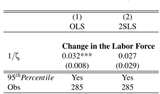
Table 2: Estimates ofζ

(1) (2)

OLS 2SLS

Change in the Labor Force 1/ζ 0.032*** 0.027

(0.008) (0.029)

95thPercentile Yes Yes

Obs 285 285

NOTES:ζis the coefficient of∆JFRkwk(1)

1+r in equation26, which uses the change in the number of workers in a industry over time

as a dependent variable and fixed effects for time and industry as controls. ∆JFRkwk(1)

1+r is the difference over time between the

product of the job finding rate and maximum wages (calculated as the 95th_{percentile) in the sector. Yearly data (from 2002 to}

2007) at the industry-level (ISIC3 2-digit) obtained from ASHE, BSD, NOMIS and LFS. Column (2) has the lag of JFRkwk(1)

1+r as

instrument. Estimates consider normalised wage values such that the average in the sample is equal to 1. Clustered standard errors at the industry-level in parentheses.∗p<0.10,∗∗p<0.05,∗∗∗p<0.01.

Column 1 shows my OLS estimates, while the second column presents the 2SLS

estimates using the lagged value JFRkwk(1) as an instrument. My estimates of ζ are

higher than the ones inArtuc, Chaudhuri, and McLaren (2010), corresponding toζ = 36.57 on column 2, the value that will be used in my counterfactuals. Indeed, in my

17_{First, from3and4I can writeU}tss1

k −Uktss0= JFRtss1

k wtssk1(1)

1+r −

JFRtss0 k wtssk 0(1)

1+r +Θ(k,t), whereJFRtkis

the job finding rate (equivalent toθt kq(θ

t

k)in my model) andw t

k(1)is the maximum wage in the sector.

model this coefficient should be higher as it captures all the labor movement frictions

between sectors, while in their paper part of the rigidity is also captured by high fixed

moving costs.18 So, using their estimates in my model would imply that workers are much more mobile than they actually are, possibly leading my real income per capita

calculations to overestimate gains (or underestimate losses).

3.1.2 Matching Function, Idiosyncratic Productivity and Vacancy Costs

I assume the following constant returns to scale matching function:

m(vt

k,utk) =m(utk)1−δ(vtk)δ.

I use the estimates fromBorowczyk-Martins, Jolivet, and Postel-Vinay(2013, Table 1), δ =0.412. To findm, I start with an estimate of 0.231 (from the same paper) and

adjust the parameter such that the probabilities of finding workers and vacancies are

always between 0 and 1. The value that will be used ism=0.19.

In all my counterfactuals I assume that idiosyncratic productivity shocks are

uni-formly distributed between zero and one (Ranjan,2012). This assumption was not used in my previous estimates. To verify the robustness of my counterfactuals to this and

other assumptions I perform additional counterfactual exercises with alternative

param-eter values.

The parameterκ, the cost of posting vacancies, is also obtained from another paper.

I consider the same value used inShimer(2005): 0.213.

3.1.3 Trade Parameters

The trade elasticity λ is estimated using a gravity equation. First, I obtain bilateral

trade flows from the World Input Output Database (WIOD).19Information on labor mar-ket characteristics by sector and country comes from the EU KLEMS dataset.20 As in Costinot, Donaldson, and Komunjer (2012), I measure the variation in productivity

18_{Another reason is that in my model this is the elasticity of employed and unemployed workers in}

the UK, while in their model they consider only employed individuals in the US. Hence, workers in their model take into account only wages when moving across sectors, while here workers also look at the probability of finding a job. Secondly, they consider average wages, while I consider the maximum wage (95thpercentile) as suggested by my model.

across countries and industries using differences in producer price indexes. Producer

price data is taken from the GGDC Productivity Level Database, which is calculated

from raw price data observations at the plant level for several thousand products (often

with hundreds of products per industry, which can be associated with varieties in my

model, as inCostinot, Donaldson, and Komunjer, 2012).21 These prices are aggregated into a producer price index at the industry level using output data. I use the inverse of

this measure as myAt_k to identify the trade elasticity.

All my gravity estimations are based on the year 2005, and 1997 lags are used as

instruments for my productivity parameter At_k (GGDC data is available only for these

two years). To compare my estimates to Costinot, Donaldson, and Komunjer(2012), I restrict my sample to the same 21 developed countries they consider plus China, and I

exclude the so called non-tradable sectors (services). I add China as an importer in all

regressions and whenever possible as an exporter since GGDC (1997) and KLEMS data

are not available for this country.

By taking logs of expression20, I obtain the following gravity equation: ln(Xk

oi) =

λln(Ak

o) +ln(Xik/Φk,i)−λln(w˜ko) +λln(dk,oi).

Following Head and Mayer (2013), I replace ln(X_ik/Φ_k,i)with an importer-product fixed effect. I do not observe ˜wk_o.22 In order to control for the last two terms of the gravity equation and still be able to identify λ as the coefficient of At_k, I replace their

values by a sector fixed effect, an exporter fixed effect, an importer-exporter fixed effect

and a 4th degree polynomial function of labor compensation, total employment, hourly

wage and labor share for each exporter-sector pair.23 So, I run the following regression at the sector-exporter-importer-level

ln(X_oik) =λln(Ak_o) + f¯_k,o+χ_ik+χ_k+χo+χoi+ε¯oi,k, (27)

where the χ are the respective fixed effects and ¯f_k,o is the 4th degree polynomial of

exporter labor market variables. ¯εoi,k is a measurement error. The results are shown in

Table3:

Controlling for labor market characteristics decreases the coefficient, while using

21_{SeeInklaar and Timmer(2008) for more details.} 22_{With the data used in the paper, ˜w}k

ocould be recovered only for the UK.

23_{Including measures for trade costs such as distance, RTA’s and common language do not change the}

Table 3: Estimates ofλ

(1) (2) (3) (4)

OLS OLS OLS 2SLS

Bilateral Trade Flows

λ 1.120*** 1.791*** 1.178*** 4.934*** (0.458) (0.471) (0.331) (1.327)

China as an Exporter Yes - -

-Labor Market Controls - - Yes Yes

Obs 6866 6194 6194 6194

NOTES:λis the coefficient of the productivity measureAk

oin equation27, which uses bilateral trade flows at the sector level as the

dependent variable and fixed effects for industry, importer-sector and exporter fixed effects. Labor Market Controls is a 4t_hdegree

polynomial function of labor compensation, total employment, hourly wage and labor share for each exporter-sector pair. Data is a cross-section of bilateral trade data in 2005 at the WIOD industry-level (roughly ISIC3 2-digit). Data obtained from WIOD, KLEMS and GGDC. Column (4) has the lag ofAko(1997 value) as instrument. Clustered standard errors at the exporter-industry level in

parentheses.∗p<0.10,∗∗p<0.05,∗∗∗p<0.01.

lagged productivity values as instruments increases it considerably. I use the value of

4.934 in my counterfactuals, which is not far fromCostinot, Donaldson, and Komunjer

(2012) estimates.

3.2

Counterfactuals

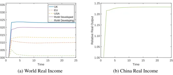
The counterfactuals performed are meant to understand how the rise of China affected

other countries in the world, especially the UK. The trade shock I have in mind is one

whereby Chinese productivity increases (Ak,CHN rises 25%) and all trade costs between

China and the rest of the world fall (dk,oCHN and dk,CHNi fall 25%) in all sectors apart

from services. This shock implies that China’s export shares around the world increases

from 0.12 to 0.2 between the two steady states. This corresponds to a growth of 64%

in China’s share of world exports, a magnitude not very different from the one observed

between 2000 (the year before China joined the WTO) and 2004 in the WIOD data

(65%). So, my shock aims to mimic the four year period following China’s entry into

the WTO in terms of percentage change in the its export share. I study how countries

respond to this shock during the transition to a new steady state.

To calculate the initial equilibrium, I use the parameters estimated in the previous

subsection. My counterfactuals also require values for worker’s labor share (βk,i) and the

size of the labor force in each country, both obtained from the WIOD - Socio Economic

Accounts.24 Labor shares are calculated as labor compensation divided by value added 24_{Available at http://www.wiod.org/new}

(at the same level as the WIOD bilateral trade data, roughly the ISIC3 2-digit industry).25 The expenditure share of each country on goods from a particular sector (µk,i) is

calcu-lated from the WIOD data. The values ofβk,i’s and µk,i’s can be seen in the Appendix,

TableB.1.

In my counterfactual exercise, I reduce the number of countries to six due to

compu-tational reasons. The “countries” chosen are China, US, UK, European Union (EU), the

Rest of the World (RoW) Developed and the RoW Developing. The last economies are

an aggregation of the remaining WIOD countries, which were separated in high-income

(Australia, Japan, Canada, South Korea and Taiwan) and low-income countries (Brazil,

India, Indonesia, Mexico, Turkey and Russia). I also aggregate the economy into five

sectors:

-Energy and Others: Energy, Mining and quarrying; Agriculture, Forestry and

fish-ing;

-Low-Tech Manufacturing: Wood products; Paper, printing and publishing; Coke and

refined petroleum; Basic and fabricated metals; Other manufacturing.

-Mid-Tech Manufacturing: Food, beverage and tobacco; Textiles; Leather and footwear;

Rubber and plastics; Non-metallic mineral products.

-High-Tech Manufacturing: Chemical products; Machinery; Electrical and optical

equipment; Transport equipment.

-Services: Utilities; Construction; Sale, maintenance and repair of motor vehicles

and motorcycles; Retail sale of fuel; Wholesale trade; Retail trade; Hotels and

restau-rants; Land transport; Water transport; Air transport; Other transport services; Post and

telecommunications; Financial, real estate and business services; Government,

educa-tion, health and other services; Households with employed persons.

The manufacturing rank of technology is based on R&D intensity in the US in 2005

from OECD STAN database. The productivity measures (Ak,i’s) are from the GGDC

database (described above). I aggregate countries and sectors using value added as

weights. The productivity parameters used in the counterfactuals are displayed in

Ta-ble B.2, which indicates that China has an absolute advantage in all the sectors. This

advantage is most likely because GGDC is based on price data, and China provides the

25_{I intentionally decrease China’s share of value added in agriculture to the second-highest value in}

cheapest goods globally. This measure does not take into account, for example, that

the UK produces higher quality goods such as airplanes and more advanced cars. Thus,

instead of estimating trade costs, I calibrate an additional parameter thatincludestrade

costs such that trade shares (π_k,oi) are as close as possible to the values observed in the

WIOD. Put another way, I substitute fordk,oi(the iceberg trade cost described previously)

in all my expressions using ¯dk,oi =dk,oi∗ωk,oi, whereωk,oi is an unobserved component

that accounts, for example, for quality difference across countries. Then, I calibrate the ¯

dk,oi’s such that trade shares are as close as possible to the ones observed in the data. The

fact that trade costs are not identified does not play a large role in my counterfactuals,

since I am interested in their relative changes (and also in relative income changes).26 In my initial steady state equilibrium, I set the unemployment benefit (bi) to a

frac-tion of the average wage in each country: UK 0.36, China 0.18, US 0.4, EU 0.5, RoW

Developed 0.5 and RoW Developing 0.14.27 These values will be fixed throughout my counterfactual exercises, as described in the model. This assumption is not innocuous.

It will imply that wages willnotabsorb all the impact from shifts in productivity/prices,

and consequently, such shocks will have an effect on the unemployment rate.

My parameterζ is held as 36.57 times the average wage in each country in the initial

equilibrium, and then kept fixed as well.28 The summary of all the parameters used are in Table4.

I am then able to find the values of Rk,i, uk,i, θk,i, ˜wk,i and Lk,i in my initial steady

state. The model performs relatively well in terms of fitting the size of the labor force in

each sector.29 26_{I also assume that ¯d}

k,oo=1 for all countries, as I am able to calibrate only relative values for ¯d’s. One

consequence of calibrating trade costs this way is that China and the RoW developing will have access to the cheapest goods in the world because they are produced by these two countries and their exporting costs are relatively high. This implies that in my initial equilibrium, the rich countries (the UK, US and Eurozone) have a high expenditure on goods around the world but not necessarily the highest real income. 27_{These values are based onMunzi and Salomaki(1999) andVodopivec and Tong(2008), for the UK,} EU, RoW Developed and China. The UK value is relatively low because much of the retained income after a job loss in the UK doesnotcome from unemployment benefits, as this is quite small (Job Seekers’ Allowance (JSA) nowadays in the UK varies between £57.35 and £113.70 per week and covers a period of approximately 6 months). The US value is based onShimer(2005), and the value of RoW developing was set slightly below that of China. In my initial steady, state unemployment rates are 0.0479, 0.0575, 0.0256, 0.0399, 0.0391 and 0.0235 in the UK, EU, China, US, RoW Developed and RoW developing, respectively. 28_{This implies that different countries will have different values for this parameters, but all the countries}

will have the same labor market frictions as the variance of the unobserved preference over sectors will be the same in each country.

29_{The labor force predicted by the model and the labor force observed in the data have a correlation of}

Table 4: Parameters used in the Counterfactuals

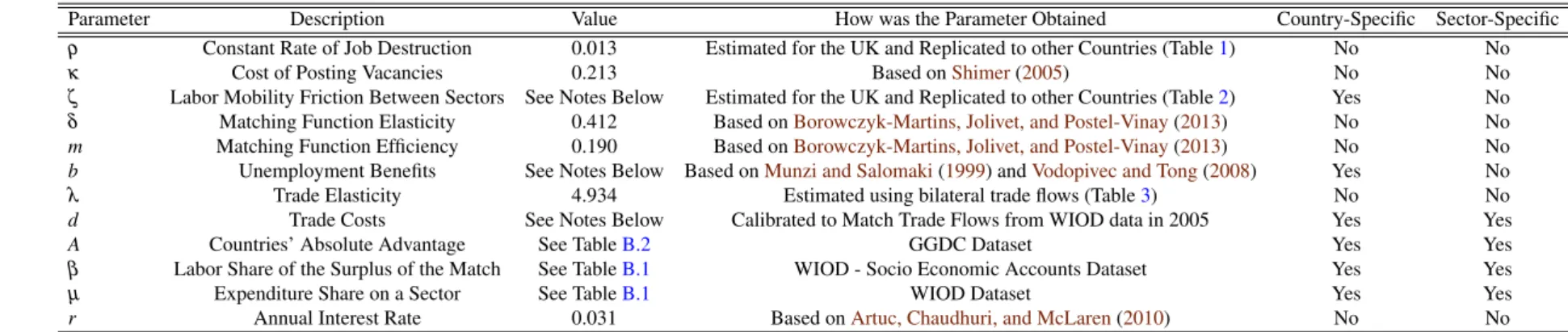
Parameter Description Value How was the Parameter Obtained Country-Specific Sector-Specific

ρ Constant Rate of Job Destruction 0.013 Estimated for the UK and Replicated to other Countries (Table1) No No

κ Cost of Posting Vacancies 0.213 Based onShimer(2005) No No

ζ Labor Mobility Friction Between Sectors See Notes Below Estimated for the UK and Replicated to other Countries (Table2) Yes No

δ Matching Function Elasticity 0.412 Based onBorowczyk-Martins, Jolivet, and Postel-Vinay(2013) No No m Matching Function Efficiency 0.190 Based onBorowczyk-Martins, Jolivet, and Postel-Vinay(2013) No No b Unemployment Benefits See Notes Below Based onMunzi and Salomaki(1999) andVodopivec and Tong(2008) Yes No

λ Trade Elasticity 4.934 Estimated using bilateral trade flows (Table3) No No d Trade Costs See Notes Below Calibrated to Match Trade Flows from WIOD data in 2005 Yes Yes A Countries’ Absolute Advantage See TableB.2 GGDC Dataset Yes Yes

β Labor Share of the Surplus of the Match See TableB.1 WIOD - Socio Economic Accounts Dataset Yes Yes

µ Expenditure Share on a Sector See TableB.1 WIOD Dataset Yes Yes r Annual Interest Rate 0.031 Based onArtuc, Chaudhuri, and McLaren(2010) No No

NOTES: Parameter values used in the main counterfactual. I additionally use unemployment benefits, expressed as a fraction of average wages in each country in the initial equilibrium: UK 0.36, China 0.18, US 0.4, EU 0.5, RoW Developed 0.5 and RoW Developing 0.14. ζ= 36.57 is also expressed as the multiple of average wages in each country in the initial equilibrium. Trade costs and other unobserved components that drive trade (such as unobserved quality of products) are calibrated such that trade flows match WIOD data in 2005, but the two terms cannot be separately observed. See also TablesB.1andB.2 for productivity components and labor and expenditure shares used in the counterfactuals.