A
T
IME
-
VARYING
M
ARKOV
-
SWITCHING MODEL FOR
ECONOMIC GROWTH
B
RUNO
M
ORIER
V
LADIMIR
K
UHL
T
ELES
Novembro
de 2011
T
T
e
e
x
x
t
t
o
o
s
s
p
p
a
a
r
r
a
a
D
TEXTO PARA DISCUSSÃO 305•NOVEMBRO DE 2011• 1
Os artigos dos Textos para Discussão da Escola de Economia de São Paulo da Fundação Getulio Vargas são de inteira responsabilidade dos autores e não refletem necessariamente a opinião da
FGV-EESP. É permitida a reprodução total ou parcial dos artigos, desde que creditada a fonte.
Escola de Economia de São Paulo da Fundação Getulio Vargas FGV-EESP
A Time-Varying Markov-Switching Model for Economic
Growth
Bruno Morier
∗Vladimir K¨uhl Teles
†November 11, 2011
Abstract
This paper investigates economic growth’s pattern of variation across and within countries using a Time-Varying Transition Matrix Markov-Switching Approach. The model developed follows the approach of Pritchett (2003) and explains the dynamics of growth based on a collection of different states, each of which has a sub-model and a growth pattern, by which countries oscillate over time. The transition matrix among the different states varies over time, depending on the conditioning variables of each country, with a linear dynamic for each state. We develop a generalization of the Diebold’s EM Algorithm and estimate an example model in a panel with a transition matrix conditioned on the quality of the institutions and the level of investment. We found three states of growth: stable growth, miraculous growth, and stagnation. The results show that the quality of the institutions is an important determinant of long-term growth, whereas the level of investment has varying roles in that it contributes positively in countries with high-quality institutions but is of little relevance in countries with medium- or poor-quality institutions.
Key-Words:Growth Regimes, Markov-Switching.
JEL Class:R14, H0.
1
Introduction
Economic growth varies among different countries and over time. Several articles attempt to explain the
differences in cross-country growth rates, showing that countries tend to converge to different growth
regimes (Desdoigts, 1999; Durlauf and Johnson, 1995; Masanjala and Papageorgiou, 2004; Tan, 2010).
Other articles show that a country can move between regimes of growth, alternating growth “miracles”
and “failures” (Easterly et al., 1993; Hausmann et al., 2004; Jerzmanowski, 2006; Jones and Olken,
2008; Pritchett, 2000, 2003). This paper proposes a methodology to study the differences in growth
rates of countries as well as the growth process changes over time employing a Markov regime-switching
approach. However, instead of considering that some countries have been fortunate to have a “good
transition probability matrix” and others are born with a “bad transition matrix”, as is usually done, we
develop a generalization of the Diebold’s EM Algorithm and estimate a Time-Varying Transition Matrix
Markov-Switching model. Thus we estimate the parameters of the transition matrix varying over time,
conditioned on the quality of the institutions and the level of investment.
The analyses performed in most studies do not incorporate all available information related to growth
and they do not consider the intertemporal factor. More recently, however, there have been several studies
that focus on precisely this aspect by dating regime changes and finding explanatory variables. In Jones
and Olken (2008), the methodology of Bai and Perron (2003) was used to date breaks in the growth
process, and a descriptive panel with means and standard deviations was included for changes in variables
correlated with growth, which was incorporated into a Solow residual model that described the anatomy
of the variations in growth. In Hausmann et al. (2004), the break for a better growth pattern (acceleration)
is analyzed. One ad-hoc criterion for acceleration was selected and calculations were performed using
means and standard deviations for the periods prior to and following the acceleration event. In Wacziarg
and Welch (2003), a similar study was performed that investigated the average impact of the removal
of restrictions on external trade on economic growth. Other studies using the same approach include
Aizenman and Spiegel (2007) and Jong-A-Pin and de Haan (2007). Although this approach explores the
intertemporal aspect, the data are not treated with a panel; in general, descriptive analyses are performed
to determine the average impact of the variables under consideration.
According to Durlauf and Johnson (1995), traditional linear regressions demand a large degree of
homogeneity in the production function among different countries, where this is always identical and
in the Cobb-Douglas format. The differences in growth patterns among countries are obvious, and the
production functions may be quite heterogeneous, which suggests the need for a more flexible approach.
in favor of a model with multiple growth regimes. In contrast to the approach in our study, the regimes
were fixed for each country, according to the initial conditions, from the beginning to the end of the
sample. This approach generated a series of literature on convergence clubs and growth regimes.
Durlauf and Johnson (1995) employed the Regression Tree technique to identify the regimes, and
other studies suggest alternative techniques using fixed regimes for each country. Hansen (2000)
de-veloped a statistical theory of threshold estimation in which the asymptotic distribution is known, thus
allowing for tests. Masanjala and Papageorgiou (2004) have used it to perform these tests, finding
non-linearity of the production function and a constant elasticity substitution (CES) format, which would be
a possible explanation for the heterogeneity of the coefficients and the existence of multiple regimes. In
Durlauf and Johnson (1995), four regimes were found. In Desdoigts (1999) and in Kourtellos (2002),
the projection pursuit technique is used to approximate the growth functions by projections on lower
dimension functions. In Alfo et al. (2008); Bloom et al. (2003); Paap et al. (2005) and Basturk et al.
(2008), the regime to which a country belongs is estimated along with the other parameters using mixture
analysis with classical statistics, and in Ardic (2006), the Bayesian statistic is used. In Canova (2004),
the predictive density technique was used. In Tan (2010), the regression tree technique is revisited with
the use of Generalized Unbiased Interaction Detection and Estimation (GUIDE)1.
The fixed regime approach, however, does not explain the inconsistencies in growth or breaks in
regimes that are characterized by the experiences of developing countries and that strongly contrast with
the experiences of the most advanced industrialized countries upon which the classical theories of
eco-nomic growth are based. In Pritchett (2000), this inconsistency is examined among the different
coun-tries, and six different growth patterns are identified to analyze the dynamic of the growth level along
with breaks and variations. In Pritchett (2003), the use of an approach with six different states of growth
through which countries pass was suggested. Each state is associated with a growth level that is
deter-mined by a different sub-model, and the growth process is then explained by toy-collection models. Thus,
the experience of inconsistency and breaks of the developing countries is explained by changes in state,
which are less common in the case of developed countries. With this approach, multiple equilibria are
permitted, such as poverty traps, heterogeneous production functions, and different roles for the
condi-tioning variables, which are non-linear and have breaks. These factors are supported by strong empirical
evidence. The changes in state are modeled probabilistically with the probabilities conditioned by the
prevailing foundations of each country. In an experiment with a constant ad-hoc transition matrix, the
author managed to recreate the dispersion of the current per capita GDP levels.
1He used GUIDE(Generalized Unbiased Interaction Detection And Estimation) based on the work of Loh (2002) who
In Jerzmanowski (2006), the approach of Pritchett (2003) was used, where a Markov-switching
model was estimated using a constant measurement of the quality of the institutions as an explanatory
variable for the transition matrix 2. The author found a positive relationship between this variable and
growth. Each state was modeled as a constant AR(1). In Kerekes (2009), the Markov-switching model
was used for the similar classification of convergence clubs, and a small number of transition matrices
that were constant and unconditioned was considered. Furthermore, each country was associated with a
matrix. Both approaches follow the proposal suggested by Pritchett (2003), although with a complexity
of the model that is considerably lower than that of the original proposal and with fewer explanatory
variables, perhaps due to the difficulties in modeling and estimating as well as a lack of data.
This work proposes a Markov-switching model with a transition matrix that is conditional to the
fundamental characteristics of each country and that varies over time. In each state, the resulting
sub-model is sub-modeled as an AR(p) with exogenous variables. The possibility that the transition matrix will
vary over time and that each sub-model will possess a linear specification with exogenous variables allows
a description that is closer to the approach of Pritchett (2003), the main contribution of this study. The
model permits:
1. Ruptures in the growth process
2. Explanatory variables that vary among countries and over time
3. Variables capable of affecting growth in various ways that are asymmetrical and non- linear (i.e.,
depending on the current state or influencing the transition among states)
4. Multiple equilibria and clubs.
Based on this model, an estimation method was developed that generalized the EM algorithm
de-scribed in Diebold et al. (1993). The original model permitted two states, with a normal, unconditional
distribution. In the model that is developed here, there are no restrictions on the number of states, and
each state is an AR(p) with exogenous variables.
Using this method, we performed estimations using an example model in which the transition
ma-trix was conditioned by the quality of the institutions and the level of investment. The primary results
indicated that the quality of the institution is an important determinant of long-term growth, whereas the
level of investment plays a differentiated role: it positively contributes towards growth in countries with
high-quality institutions but is of little relevance in countries with medium- or poor-quality institutions.
2
This study is organized as follows. The next section presents the model. Section 3 presents the
estimation algorithm. Section 4 presents the empirical model and discusses the results. Finally, Section 5
concludes and opens a discussion for future studies.
2
The Model
In this section, we present the general model with regime changes for growth. Consider a generic country
c. Letgct be the growth rate for country cbetween time t−1 andt. gct is modeled following a Time-Varying Markov-switching process withSAR(p) states. The precise meaning is that for each timetthat
countrycis in an (unobserved) statesct ∈ {0,· · · , S−1}, sct follows a Markov process with S states, and in each state,gctfollows a different AR(p) process.
The exogenous variables may affect the growth process through the distribution of each AR(p) state
or based on a transition matrix of the Markov process ofsct. Letzct = (zict)i=1...Nz be the vector of theNz
exogenous variables that affect the growth process in each AR(p) state withz1ct = 1. The same variables
influence the growth of each country even though the value of these variables varies withc andt. For
each state, the AR(p) process is given by the expression:
gct =
Xp
i=1
αisctL
i·g ct+
Nz
X
i=1
γisct ·z
ct i
+ǫct
with ǫct ∼N(0, σ2sct) (i.i.d.)
(1)
The coefficients(α, γ) = ({αisct},{γisct})are dependent on the given state. αdetermines the degree
to which the current growth is affected by the previous growth, thus constituting the only memory in the
model beyond the previous statest−1. γ represents the degree to which each variable zi influences the
growth in each state. Finally,σ= ({σsct})determines the standard deviation of each state.
The dynamics ofsctare given by a Markov process with a transition matrix that varies over time and
is conditional on exogenous explanatory variables. TheseNx conditional variables are collected in the
vectorxct= (xcti )i=1...Nx withx1ct = 1. We can write:
P(sct=i|sct−1 =j) = pij(xct) (2)
pij(xct) =
exp(βijxct)
1 + S−2
X
k=0
exp(βkjxct)
, ifi= 0,· · · , S−2
1−
S−2
X
k=0
pkj(xct) , ifi=S−1
(3)
The coefficients β = {βij}determine how each exogenous variable in xk influences the probability of transition between statesiandj. Eachβij is a vector(Nx×1).
Note that this is a flexible model, with the explanatory variables conditioning the process of each
state and the transition matrix. It is more realistic than the usual Markov-switching specification with
a fixed matrix (as in Hamilton (1994)), as it allows the fundamental characteristics of each country to
influence the dynamics of the state. It is reasonable to assume, for example, that the probability of a crisis
in a country with good institutions and good macroeconomic policies is less than that in a country with
poor institutions and policies. The fundamental characteristic may change over time, as is the case with
investment and the political regime.
We now develop the immediate results of the model. Denoting Pct = Pct(xct) as a matrix with
coefficients pij(xct) and denoting sˆct =
P(sct = 0|θˆ), . . . , P(sct = S −1|θˆ)
′
as the probability of
occurrence for each state for some information setθˆ, we achieve the following results:
ˆ
sct =Pctˆsct−1 (4)
given by the Markov property ofsct.Long-term growth is well-defined for each state if zi are stationary
and the coefficients do not imply a unit root. In this case, denotingµzi =E[zi]as the expectation for each
exogenous variable, the long-term growth for each statestis given by
Long Run Growth ofsct :E[gct|sct =j] = Nz
X
i=1
γijµzi
1− p X i=1 αij (5)
Maintaining the transition matrix Pct constant (which can be interpreted as maintaining the same
policies and the status quo), we can use equation (4) to derive the unconditional probabilities for each
state. Usingπ = (π0,· · · , πS−1)′as the unconditional probability, equation (4) impliesπ =Pctπ. We also haveX
i
πi = 1. As in Hamilton (1994), the solution to this system is given by
π= (A′A)−1Ae
where denotes theS+ 1column of the identity matrixIS+1 and where
A
(S+1 X S)’ =
IS−Pct
1· · ·1
(7)
In this case, we can use equations (5) and (6) to calculate the long-term growth of the economy of
countrycwith
E[gct] = S−1
X
i=0
E[gct|st=i]πi (8)
3
Estimation Method
In this section, we extend the algorithm from Diebold et al. (1993) for the model described in the previous
section. The algorithm is based on the expectation maximization technique, which is flexible and
appro-priate for new extensions. A discussion on the EM algorithm can be found in Dempster et al. (1977),
Watson (1983), and Ruud (1991). We can cite other Markov-switching algorithms with EM: Hamilton
(1990), Durland and McCurdy (1994), and Filardo (1994).
Following the model described in the previous section, the data available for the estimation should be
gct, zct, andxct. We assume that these data are available between t = 1and t = T. From here on, we
will use underlined notation to indicate the collection of all the data available for one variable up until the
time index such thatxcT = (xc1, . . . , xct). Thus, the input for the estimation isgcT, xcT, zcT.
Letρc
j = P(sc1 = j),ρc = (ρc0, . . . , ρcS−1)andρ = ({ρ
c}). The state of each country,s
ct, is hidden,
and the probability of occurrence of each state follows the dynamics described in (4). Thus, the joint
distribution ofsctis determined byρcand by the transition matrixPct.
The parameters for the estimation are collected inθ =α, β, γ, σ, ρ
. These will be the final output of
the estimation algorithm. If statessctwere known, we could simply estimate the complete data function
of maximum likelihood to obtain estimations for the parameters of the model. Even though this is not the
case, the calculation of this function proves to be useful. The function will be calculated by iterating a
dynamic model following equation (4) and using the conditional distribution for each state given in (1).
As the growth of each country in the model is independent, we will first set a countrycand calculate its
function of maximum likelihood. For a lighter notation, we will removec, usinggtinstead ofgct. We then
f(gT, sT|xT, zT, θ) = f(g1, s1|xT, zT, θ) T
Y
t=2
f(gt, st|gt
−1, st−1, xT, zT, θ)
= f(g1|s1, xT, zT, θ)P(s1) T
Y
t=2
f(gt|st, gt−1, xT, zT, θ)P(st|st−1, gt−1, xt−1, zt−1, θ)
= f(g1|s1, z1, θ)P(s1) T
Y
t=2
f(gt|st, gt
−1, zt, θ)P(st|st−1, xt, θ) (9)
wheref is the probability density given by (1) such that
f(gt|st=j, gt
−1, zt, θ) = 1
q
2πσ2 j exp
− gt−
Xp
i=1
αistL
i ·gt−
Nz
X
i=1
γist ·zit
!2
2σ2 j (10)
We can use equations (4), (9), and (10) to calculate the complete-data function of maximum likelihood
for a country. We can further express this function of maximum likelihood in terms of an indicator
function, separating the possible realizations of the states for each timet. Thus, we obtain
f(g
T, sT|xT, zT, θ) = S−1
X
j=0
f(g1|s1 =j, z1, θ)ρjI(s1 =j) T
Y
t=2 S−1
X
j1=0
S−1
X
j2=0
I(st =j1, st−1 =j2)
× f(gt|st =j1, gt−1, zt, θ)P(st=j1|st−1 =j2, xt, θ)
(11)
whereρj =P(s1 =j)is thej-th coordinate ofρand the indicator functionI is1if the condition is true
and0 if it is not. Then, applying the logarithm and the expectation operator E[.] in equation (11), we
obtain
Ehlogf(g
T, sT|xT, zT, θ)
i
= S−1
X
j=0
ρj logf(g1|s1 =j, z1, θ) + logρj
+ T
X
t=2 S−1
X
j1=0 S−1
X
j2=0
P(st =j1, st−1 =j2|gT, xT, zT, θ)
× nlogf(gt|st=j1, gt
−1, zt, θ) + logP(st =j1|st−1 =j2, xt, θ)
o
(12)
We observe that the operator, E[.], essentially substitutes I(.) for P(.) in the equation. Using the
of the functions of log maximum likelihood for each country. LetΨbe this function andψc be the log
function of maximum likelihood for each country. We then have
Ψ =X
c
Ψc =X
c S−1
X
j=0
ρj logf(gc1|sc1 =j, zc1, θ) + logρcj
+ X
c T
X
t=2 S−1
X
j1=0
S−1
X
j2=0
P(sct =j1, sct−1 =j2|gcT, xcT, zcT, θ)
× nlogf(gct|sct =j1, gct
−1, z
ct, θ) + logP(s
ct =j1|sct−1 =j2, x ct, θ)o
(13)
The last equation is the basis of the estimation procedure. We did not compute the complete maximum
likelihood function, as we did not observe the states that were realized. However, this last equation for
the expectancy of the complete function of maximum likelihood can be estimated. The parameters inθ
will be estimated by maximizing equation (13).
3.1
EM Algorithm - General Procedure
Given the model from Section 2, we have created formulae for all of the terms of equation (13) with the
exception ofP(sct =j1, sct−1 =j2|gcT, xcT, zcT, θ). This last term refers to the smoothed probability of occurrence of statessct = j1, sct−1 =j2 that is conditional on all of the data previous and subsequent to
timet. We can obtain this term algorithmically. Because this term is conditional on all of the data, this
term tends to have variations that are lower than those of the other terms of the equation for values ofθ
that are close to the maximum function of expected maximum likelihood.
The concept of optimization then emerges in two stages, in which the equation (13) is maximized by
maintaining the smoothed probabilities constant.
(1) Select aθ(0)
(2) With the lastθ(l)available, calculate
P(st =j1, st−1 =j2|gT, xT, zT, θ(l))para(j1, j2)∈(0, . . . , S−1)2 et∈(2, . . . , T) (3) Calculateθ(l+1) = arg max
θ E
h
logfl(gT, sT|xT, zT, θ)i (4) If||θ(l+1)−θ(l)||> ǫ, then return to step (2)
whereǫand the||.||norm define a convergence criterion. flfrom stage (3) is obtained via the smoothed probabilities calculated with the lastθ(l)available, i.e., by substitutingP(s
ct =j1, sct−1 =j2|gcT, xcT, zcT, θ) byP(sct =j1, sct−1 =j2|gcT, xcT, zcT, θ(l))Stage (2) is called the expectation step and stage (3) is called the maximization step. When there is convergence, the θ found by the procedure will be a numeric
3.2
Expectation Step
The algorithm described here calculates the smoothed probabilities of the occurrence ofsct=j1, sct−1 =
j2 for all pairs(j1, j2)with an optimization as described in Diebold et al. (1993). Again, we will treat
each country separately, removingcfrom the notation.
1. Pre-calculus
(a) Use equation (10) to calculatef(gt|st, gt
−1, xt, zt, θ
(l)) = f(g t|st, gt
−1, zt, θ (l))for
(t, st)∈(1, . . . , T)×(0, . . . , S−1).
(b) Use equation (3) to calculate the matrixPkt
2. Calculate the filtered probabilities3P(st, st−1|gt, xt, zt, θ(l))for(st, st−1)∈(0, . . . , S−1)2 and
t ∈(2, . . . , T)
(a) Calculatef(gt, st, st−1|gt−1, xt, zt, θ(l))
Fort= 2, we use the identity
f(g2, s2, s1|g1, x2, z2, θ(l)) =f(g2|s2, g1, x2, z2, θ(l))
| {z }
Step 1
P(s2|s1, g1, x2, z2, θ(l))
| {z }
Step 1
P(s1) | {z }
ρs
1
(14)
Fort= 3. . . T, we use the identity
f(gt, st, st−1|gt−1, xt, zt, θ(l)) = S−1
X
st−2=0
f(gt|st, gt−1, xt, zt, θ(l))
| {z }
Step 1
P(st|st−1, gt−1, xt, zt, θ(l))
| {z }
Step 1
P(st−1, st−2|gt−1, xt, zt, θ(l))
| {z }
Step 2.a above
(15)
(b) Calculate the probability density ofgt:
f(gt|gt
−1, xt, zt, θ (l)) =
S−1
X
st=0
S−1
X
st
−1=0
f(gt, st, st−1|gt−1, xt, zt, θ(
l)) (16)
(c) The filtered probabilities are obtained for timet
P(st, st−1|gt, xt, zt, θ
(l)) = f(gt, st, st−1|gt−1, xt, zt, θ
(l))
f(gt|gt
−1, xt, zt, θ
(l)) (17)
3. Calculate the smoothed probabilitiesP(st, st−1|gT, xT, zT, θ(l))to(st, st−1)∈(0, . . . , S−1)2and
t ∈(2, . . . , T)
3
(a) For each timet∈(2, . . . , T)and each pair(st, st−1)∈(0, . . . , S−1)2 sequentially calculate
P(sτ, sτ−1, st, st−1|gt−1, xt−1, zt−1, θ
(l))for allτ ∈(t+ 2, . . . , T)Forτ =t+ 1, we use the identity
P(st+1, st, st−1|gt+1, xt+1, zt+1, θ(l)) =
f(gt+1|st+1, gt, xt+1, zt+1, θ(l))P(st+1|st, gt, xt+1, zt+1, θ(l))P(st, st−1|gt, xt+1, zt+1, θ(l))
f(gt+1|gt, xt+1, zt+1, θ(l))
(18)
where the first two terms of the numerator were obtained from the first step, the third term was
obtained from step 2(c), and the denominator was obtained from step 2(b).
Forτ ∈(t+ 2, . . . , T), we use the identity
P(sτ, sτ−1, st, st−1|gτ, xτ, zτ, θ(l)) = S−1
X
sτ−2=0
f(gτ|sτ, gτ−1, xτ, zτ, θ( l))
×P(sτ|sτ−1, gτ−1, xτ, zτ−1, θ
(l))P(s
τ−1, sτ−2, st, st−1|gτ−1, xτ, zτ, θ(l))
f(gτ|gτ
−1, xτ, zτ, θ
(l))
(19)
where the first two terms of the numerator were obtained in the first step, the third term of the
numerator was obtained from step 3(a), and the denominator was obtained from step 2(b).
(b) Calculate the smoothed probabilities for timet
P(st, st−1|gT, xT, zT, θ( l)) =
S−1
X
sT=0
S−1
X
sT−1=0
P(sT, sT−1, st, st−1|gT, xT, zT, θ(
l)) (20)
3.3
Maximization Step
To maximize equation (13), we will compute the first-order conditions in relation to (α, β, γ, σ). As
suggested in Hamilton (1994) for a model with a fixedPct, we calculate ρ from equation (6), i.e., as
the long-term expectation for the probability of occurrence of each state given the conditions of the
exogenous variables and the current estimation ofβ. BecausePctvaries in this model, the option is given
Let
Ψl = Ehlogfl(gT, sT|xT, zT, θ)i
ϕctj = logf(gct|sct =j, gct −1, z
ct, θ )
ξjct1,j2 = P(sct=j1, sct−1 =j2|gcT, xcT, zcT, θ(l))
ξjct = P(sct=j|gcT, xcT, zcT, θ(l))
pctj1,j2 = P(sct=j1|sct−1 =j2, xct, θ)
Γctj = gct−
Xp
i=1
αi,jLi
·gct−
Nz
X
i=1
γi,j·zict
(21)
We observe that theξ’s are constant in relation to the(α, β, γ, σ), which are estimates. This
relation-ship is given by
ξjct=
S−1
X
j2=0
ξjct1,j2 , ift >1
ρc
j , ift= 1
(22)
Applyinglogin equation (10), we obtain
ϕctj = −
Γct j
2 2σj2 −
log 2πσ2j
2 (23)
Using equation (22) and the above definitions (21), we have a simpler representation forΨl derived
from equation (13), and the substitution of the dependent smoothed probabilities onθbyθ(l).
Ψl = X
c S−1
X
j=0
ρj ϕctj + logρ c j +X c T X t=2 S−1
X
j1=0
S−1
X
j2=0
ξctj1,j2 ϕjct+ logpctj1,j2
= X
c,t,j
ξjctϕctj +X c,j
ρcjlogρcj+ T
X
t=2
X
c,j1,j2
ξjct1,j2logpctj1,j2 (24)
In the second line of the last equation, we have a representation in which the first term is a function of
(α, γ, σ), the second is a function ofρ, and the third is a function ofβ.
Deriving equation (23), we have ∂ϕct j1 ∂αk,j =
LkgctΓct j
σ2 j
, ifj1 =j
0 , ifj1 6=j
(25) ∂ϕct j1 ∂γk,j = zct kΓctj
σ2j , ifj1 =j
0 , ifj1 6=j
(26)
Deriving equation (24) and substituting equations (25) and (26), we obtain the first-order conditions
∂Ψl
∂αk,j =
X
c,t
ξjctLkgct
"
gct−
Xp
i=1
αi,jLi
·gct−
Nz
X
i=1
γi,j·zcti
#
σ2 j
= 0 (27)
∂Ψl
∂γk,j =
X
c,t
ξjctzkct
"
gct−
Xp
i=1
αi,jLi
·gct−
Nz
X
i=1
γi,j ·zict
#
σ2j = 0 (28)
Rearranging the last equation, we obtain
p X i=1 " X c,t
ξjct(Lkgct)(Ligct)
#
·αi,j+ Nz X i=1 " X c,t
ξjct(Lkgct)zict
#
·γi,j =
X
c,t
ξjct(Lkgct)gt (29)
p X i=1 " X c,t
ξjctzkct(Ligct)
#
·αi,j + Nz X i=1 " X c,t
ξjctzkctzict
#
·γi,j =
X
c,t
ξctj zkctgct (30)
For each fixed j, we have a linear system with variables(αi,j, γi,j), withp+Nz variables, and with
p+Nz equations (varying the k in the two equations). (αi,j, γi,j)are calculated by resolving this
system.
2. Calculation ofσ
Deriving equation (23), we obtain
∂ϕct j1 ∂σj = Γct j 2 σ3 j − 1 σj
, ifj1 =j
0 , ifj1 6=j
Deriving equation (24) and substituting equations (31), we obtain the first-order conditions
∂Ψl
∂σj
=X
c,t
ξjct· Γ ct j 2 σ3 j − 1 σj !
= 0 (32)
The volatilities of each state may then be calculated with
σj =
X
c,t
ξjct Γct j
2
X
c,t
ξjct
(33)
3. Calculation ofβ
Deriving equation (24), we obtain
∂Ψ
∂βi1,i2
= T X t=2 X c,j2 ∂ ∂βi1,i2
S−1
X
j1=0
ξctj1,j2logpctj1,j2 (34)
Note that
1−
S−2
X
k=0
pctk,j2 = 1 + S−2
X
k=0
exp(βk,j2x
ct )
!−1
∂ ∂βi1,i2
log 1 +
S−2
X
k=0
exp(βk,i2x
ct)
!
=xctpcti1,i2
(35)
We can expand the term that is derived using equation (3). Using the first identity of equation (35)
S−1
X
j1=0
ξjct1,j2logpctj1,j2 = S−2
X
j1=0
ξjct1,j2log
exp(βj1,j2x
ct)
1 + S−1
X
k=0
exp(βk,j2x
ct )
+ξSct−1,j2log 1− S−2
X
k=0
pctk,j2
!
= S−2
X
j1=0
ξjct1,j2βj1,j2x
ct−ξct
j2log 1 +
S−2
X
k=0
exp(βk,j2x
ct)
!
(36)
Substituting this into equation (34) and using the second identity of equation (35), we obtain the
first-order condition
∂Ψl
∂βi1,i2
=X
c T
X
t=2
xct ξict1,i2−ξct−1 i2 p
ct i1,i2
= 0 (37)
arising from probabilities expressed in logit form. We can, however, approximate pct
i1,i2 in a
first-order Taylor series from β(l) in a manner that is analogous to that of Diebold et al. (1993). This
approximation will be especially good as we approach the convergence criterion, i.e., the realβ.
pcti1,i2 =pcti1,i2(βi1,i2) =p
ct i1,i2(β
(l)) +φct
i1,i2·(βi1,i2 −β
(l) i1,i2)
′ (38)
wherepct
i1,i2(.)designates the probability of transition in the function ofp
ct
i1,i2 as in equation (3). The
derivative is given by
φcti1,i2 = ∂p ct i1,i2
∂βi1,i2
(β(l)) = ∂
∂βi1,i2
exp(βi1,i2x
ct)
1 + S−1
X
k=0
exp(βk,i2xct)
= (xct)′pct i1,i2(β
(l))−pct i1,i2(β
(l))2
(39)
Substituting equation (38) into equation (37) and rearranging, we obtain
βi1,i2 =β
(l) i1,i2 +
" X
c,t
xctξct−1 i2 φ
ct i1,i2
#−1"
X
c,t
xct ξict1,i2 −ξct−1 i2 p
ct i1,i2(β
(l))
#
(40)
with which we can calculate the Beta.
4
Empirical Model
In this section, we use the general model and the estimation algorithm developed in the last two sections
to estimate an exemplary empirical model with a transition matrix that varies over time and that is
con-ditioned by the quality of the institutions and by the level of investment (%GDP). Each state is modeled
following an AR(1) without explanatory exogenous variables.
The resulting model possesses three states, which is one less than is found in Jerzmanowski (2006).
We are unaware of the objective statistical criterion in the literature for the selection of the number of
states in Markov-switching models similar to the one used in this work. However, the selection is made
because, with one variable and the conditioning from the transition probabilities, the estimated model with
four states appears to require too much of the available data; i.e., its resulting transition matrix presents
many cases of 100% or 0% transition probability, indicating few occurrences of transition conditional on
Despite having one less state, the results corroborate those of the model of Jerzmanowski (2006) with
virtually the same first three states from that model: stable growth, miraculous growth, and stagnation.
The only differences appear to be that the stagnation state in this work is actually a mix of the crisis
and stagnation states from Jerzmanowski (2006) because of the greater volatility that is presented. The
resulting model can be seen as a test of the robustness for the result of Jerzmanowski (2006), as the
results are analogous to the introduction of investment with a different data set: the author’s data were
from 89 countries during a period from 1962 to 1994 with a Penn World Tables 6.1.
We can compare the states that were found with the six states that were established in an exogenous
and ad-hoc manner in Pritchett (2003). Stable growth appears to be equivalent to the union of “steady
growth at levels of income near world leaders” and the “non-converging steady growth” state. The
mirac-ulous growth state corresponds to the rapid growth state. The stagnation state corresponds to the poverty
trap, non-poverty trap stagnation, and growth implosion states.
4.1
Data
Data from 73 countries between 1962 and 2007 were considered4
To measure the quality of the institutions, we used the index of government anti-diversion policies
(GADP) from Hall and Jones (1999) and Jerzmanowski (2006). This index follows the same principle
as the index found in Knack and Keefer (1995) and combines a measurement of the observance of laws,
risk of expropriation, corruption, and the quality of the bureaucracy, among others. The index is assumed
to be constant over the time period, varying only by country, as in Jerzmanowski (2006). This variable
will be denoted as GADPc.
To measure the level of investment, we use the Gross fixed capital formation (GFCF) from the World
Bank database (WDI). For each timet, the conditioning variable of the transition matrix is the mean of
the GFCF for the five previous years(t−5, . . . , t−1). For some countries in the sample, an extrapolation for the initial years was performed due to the lack of data. However, the GFCF series exhibits slow
changes during this time, and even considering that the series used is the average of 5 years, we should
not be biased by the procedure that was adopted. From this point on, this variable (average GFCF of the
5 previous lags) will be denoted by GFCFct. For economic growth, the per capita GDP growth from the
Penn World Tables (PWT), version 6.3, was used.
4Estimates of the Probability Matrix exhibit only small variations over time. Thus, although the data are annual, we
4.2
Results
In this subsection, we discuss the results. We begin with the main results of the estimation (estimated
parameters), and in the sequence, we present a brief discussion with examples from specific countries.
Table 1: States: AR(1) Process
Constant AR[1] Volatility Growth
(γ1j) (α1j) (σj) Long Term
State 1 1.27 0.35 2.42 1.97
State 2 4.20 0.30 3.46 6.03
State 3 0.15 0.04 6.47 0.16
Table 1 presents the parameters of the AR(1) process described in equation (1) for each state j =
(1,2,3). The first column shows the constant term (γ1j), the second column shows the coefficient of lag
1 (α1j), and the third column shows the volatility (σj). Long-term growth is calculated with (5).
State 1, which we call stable growth, is the state that best represents the experience of the
devel-oped countries with a growth rate close to 2%, a high auto-correlation among the growth rates, and low
volatility. Countries such as Colombia and Pakistan with stable and non-convergent growth as defined in
Pritchett (2003) also fit into this category.
State 2, which we call miraculous growth, is a state that tends to have a short duration in most countries
and consists mostly of “catch-ups” in growth by less developed countries. In the historical data that are
available, the countries that maintained this state for the longest period of time are the emerging Asian
countries, with illustrative cases such as Japan and China.
State 3, which we call stagnation, is most frequent among emerging countries that fail to achieve
convergence and among poor African countries. It is a highly persistent state for the poorest countries
and has very high volatility; countries in this state achieve some years of strong growth, but they generally
end up with years of negative growth and the average growth is quite low.
Tables 2,3,4 present the most important examples of countries and periods of incidence for each of
the states. The incidence of each state in these tables follows the convention with a probability greater
than 75% for the occurrence of the state. The variables of GADP and GFCF are included, with values that
are normalized to the mean and standard deviation for the entire sample, including all countries (standard
score). The GFCF value of each country presented in the table is the mean of the GFCF normalized for
the period in which the state in question occurs.
The criterion for the formation of table 2 was countries with 30 years or more in state 1, summing
Table 2: Main countries and periods of incidence of State 1
Country GADP GFCF Periods
Australia 1.29 0.74
1962-Austria 1.38 0.46 1962-1975
1981-Belgium 1.40 0.42
1962-Bolivia - 1.25 - 0.73 1972-1980
1986-Canada 1.50 - 0.01 1962-1981
1984-Switzerland 1.61 0.89 1962-1974
1978-Colombia - 0.40 - 0.40
1963-Costa Rica 0.09 - 0.30 1963-1979
1985-Denmark 1.54 0.03
1965-Spain 0.70 0.38
1974-Finland 1.52 0.50 1962-1967 1973-1990
1996-France 1.34 0.12
1962-United Kingdom 1.30 - 0.43
1962-Greece 0.28 0.78
1977-India - 0.28 - 0.01 1972-1998
2000-Israel 0.49 0.23
1975-Italy 0.76 0.03 1963-1971
1980-Japan 1.30 1.09
1977-Sri Lanka - 0.87 0.04 1963-1971
1981-Netherlands 1.56 0.23
1962-Norway 1.46 0.79
1962-New Zealand 1.55 0.21 1962-1966
1978-Pakistan - 0.91 - 0.58 1963-1968
1973-El Salvador - 1.29 - 0.93 1963-1977
1983-Sweden 1.55 0.01
1962-United States 1.37 - 0.37
1962-South Africa 0.41 0.01
1963-Mean 0.72 0.12
Table 3: Main countries and periods of incidence of State 2
Country GADP GFCF Periods
Brazil 0.14 - 0.08 1968-1978
Chile - 0.02 - 0.28 1977-1979 1986-1995
China Version 1 - 0.05 1.89
1971-Greece 0.28 3.40 1963-1973
Hong Kong 0.65 0.66 1963-1988
1999-Indonesia - 0.77 - 0.72 1969-1979
Japan 1.30 1.96 1963-1973
Korea, Republic of 0.39 0.75 1963-1979 1982-1996
Malaysia 0.17 0.73 1973-1980 1987-1996
Portugal 0.74 0.61 1963-1973 1976-1977 1986-1988
Singapore 0.96 1.75 1965-2003
Thailand 0.28 0.87 1966-1995
Table 4: Main countries and periods of incidence of State 3
Country GADP GFCF Periods
Argentina - 0.33 0.05 1963-1966 1978-1991 1999-2002
Central African Republic - 1.07 - 1.11 1967-1997
Cote d‘Ivoire - 0.11 - 0.46 1964-1968 1979-1993
Fiji - 0.18 - 0.21 1965-1968 1973-1975 1978-2000
Gambia, The - 0.38 - 0.91 1966-1967 1970-1972 1974-1983 1990-2001
Honduras - 1.05 - 0.08 1969-1971 1978-1988 1990-1995 1998-2000
Iran - 0.76 0.56 1974-1995
Mali - 1.57 - 0.66 1963-1990 1994-1997
Niger - 0.63 - 1.38 1963-2004
Senegal - 0.76 - 1.37 1963-1985
Togo - 0.95 - 0.18 1970-2003
Trinidad &Tobago - 0.16 0.23 1968-1994
Venezuela - 0.18 0.47 1974-2004
Congo, Dem. Rep. - 1.97 - 1.48 1963-2005
Mean - 0.72 - 0.47
a relationship between this variable and the occurrence of stable growth. In addition, most countries
that do not have a high GADP have episodes where there is a deviation from this state. Some of these
countries, such as Colombia, Pakistan, and India prior to 1999, are explicitly classified as “stable and
non-convergent growth” by Pritchett (2003). This also appears to be the case for the other countries
with a below-average GADP. The table does not reveal a strong relationship between the GFCF and the
occurrence of state 1.
Table 3 shows countries with 10 years or more in state 2, summing all episodes. We observe in
table 3 that the mean GFCF is high, i.e., 0.96, indicating a relationship between this variable and the
occurrence of miraculous growth. In addition, most of the countries that do not possess a high GFCF
maintain miraculous growth for a few years. The Asian countries tend to maintain this type of growth.
Greece decreased its rate of investment after the occurrence of this state. Japan reached convergence of its
per capita GDP with that of the leading countries, concluding the “catch-up” phase and beginning stable
growth after a transition period of stagnation. The GADP was also above average. The exception of the
table appears to be Indonesia, which had a single miraculous growth event that lasted 10 years.
Table 4 shows countries with 20 years or more in state 3, summing all episodes. We observe in table 4
that the mean GFCF and mean GADP are low, at−0.72and−0.47, marking a relationship between these variables and the occurrence of stagnation.
4.2.1 The Role of the Quality of the Institutions and of Investment
In this subsection, we explain the relationships among the quality of the institutions, investment, and
Figure 1: The Impact of Investment for Countries with a High Quality of Institutions
Note: Normalized GADP set at 1.2.
Figure 2: The Impact of Investment for Countries with a High Quality of Institutions
Note: Normalized GADP set at 1.2.
complete description of the impact of each variable than does a purely linear model. As two variables are
under consideration, we first normalized the level of the institutions in three levels(−1.2,0,1.2), and we analyzed the impact of investment for each one of these levels. The levels were selected for observation
of the dynamics not only for countries with average institutions but also for those with good or poor
institutions. The selected levels correspond approximately to the 10% and 90% percentiles. Next, we
established the same three levels for investment for a similar analysis.
In figure 1, we observe the impact of investment for countries with high-quality institutions. The graph
on the left shows the ergodic growth (long-term) and the one on the right shows the ergodic probabilities
(unconditional) of occurrence for each state. These are calculated from equations (5), (6) and (8). We
Figure 3: The Impact of Investment for Countries with Average-Quality Institutions
Note: Normalized GADP set at 0.
Figure 4: The Impact of Investment for Countries with Low-Quality Institutions
Note: Normalized GADP set at -1.2.
amount of time allocated to the miraculous growth state, thus generating greater long-term growth.
Figure 2 explains the changes in the transition matrix caused by the variations in the levels of
invest-ment. Each graph indicates the probability of occurrence of each state int+ 1 and conditional on the
current state int. We observe that the greatest impact of investment is found on the maintenance of
mirac-ulous growth (first graph) with no relevant role for the other situations. The probability of maintaining
this growth goes from 53% for the countries with the least amount of investment to approximately 75%
for those countries with the greatest amount of investment.
Figure 3 shows the case of medium-quality institutions. In this case, an increase in investment does
not significantly impact growth. The effect even appears to be slightly negative due to the amount of time
in stagnation. However, the effect appears to be somewhat irrelevant, generating a variation of 0.3% from
end to end in the level of investment. We also observe that, for this level of institution quality, miraculous
growth is frequent and is counterbalanced in terms of the average growth by the stagnations, which are
also frequent. The growth is then more volatile than in the previous case, and a significant portion of the
incidence of miraculous growth is due to the “catch-ups” from previous stagnations and not “catch-ups”
Figure 5: The Impact of Institutions for High-Investment Countries
Note: Normalized GFCF set at 1.2.
Lastly, in figure 4, we have the case of below-average institution quality. In this case, the growth
dynamics are not favorable, and the level of investment does not have a positive effect. The effect is
irrelevant, is less than in the previous case, and even tends to be negative. We continue with the analysis
of a fixed level of investment. In figure 5, we have a dynamic for a high level of investment. We observe
that the ergodic growth is increasing in most of the graph and that the institutions exert a strong impact
over growth. In general, better institutions increase the occurrence of miraculous growth and decrease
stagnation.
The exception is found for the final plot above 0.7 in the level of institution quality, where there is a
decline in miraculous growth. This effect, which also occurs in the model of Jerzmanowski (2006), is
given by the correlation between the high quality of the institutions and the per capita GDP level. In the
sample, there is a concentration of countries with a high per capita GDP level among the countries with
institutions of very high quality, and this high per capita GDP level decreases the incidence of miraculous
growth. According to Pritchett (2003), this is due to the “catch-up” in growth convergence.
Following the reasoning of Pritchett (2003), a possible explanation for the correlation between the
institution level and the per capita GDP of the sample is that the initial conditions of the per capita GDP
are given by the accumulated growth up until the beginning of the sample and with the institution quality
as a variable that is related to growth. The accumulated growth is influenced by that variable. However,
it is logical to include the per capita GDP in the transition matrix, although perhaps only in the transition
from the miraculous growth state.
In figure 6, we have a transition matrix with a high level of investment for the function of the quality
of the institutions. We can find the reasons for a lesser amount of time in stagnation in the first two tables.
When in stagnation, the economy with better institutions has an increased chance of recovery and moving
into miraculous growth, whereas the countries with poor-quality institutions have a high probability of
Figure 6: The Impact of the Institutions for High-Investment Countries
Note: Normalized GFCF set at 1.2.
Figure 7: The Impact of Institutions for Medium-Investment Countries
Note: Normalized GFCF set at 0.
institutions has greater stability, whereas the economy with worse institutions has a greater chance of
falling into stagnation, even though there is a long period during which it maintains stable growth. The
third table shows this effect, which has been discussed previously: miraculous growth continues for a
shorter period of time, segueing into stable growth. We observe that the increase in the probability of
stagnation is minimal and immaterial as the incidence of stagnation in the highest levels of institution
quality is not perennial, and it is more likely that miraculous growth will occur, where this will occur
even more quickly as the level of the institutions increases.
In figures 7 and 8, we have the case of average and below-average levels of investment. The dynamic
is similar to that discussed in the case of above-average investment but with smaller oscillations in the
Figure 8: The Impact of Investment for Low-Investment Countries
Note: Normalized GFCF set at -1.2.
Figure 9: Growth and the Occurrence of the States for Brazil
4.2.2 Cases of Selected Countries
In this section, we present the states that are attributed by the model to six selected countries: Brazil,
Argentina, China, Japan, the United States, and the Congo. The objective is to use practical cases to
indicate how the change of regimes works and to show that certain factors may impact these changes.
The model seeks to explain the probabilities of change conditional to the structural variables, but most of
the changes have cyclical and specific aspects that lead to the transition.
In figure 9, we examine the case of Brazil. In the 1960s and the 1970s, we have a dominant
prob-ability of miraculous growth. Despite the rising debt and the troubled political and social scenes that
characterized this period, there was strong growth spurred by investment, particularly in infrastructure. In
the 1980s, the effects of the oil crisis, which occurred before the 1980s, could no longer be circumvented.
Figure 10: Growth and the Occurrence of the States for Argentina
Figure 11: Growth and the Occurrence of the States for China
excesses in the external and fiscal accounts and, furthermore, had to control for inflation; all of this
oc-curred at a time of transition in the political regime with the end of the dictatorship. After the constitution
of 1988 and the control of inflation, there was stabilization of growth at a non-convergent stable state, to
apply the terminology of Pritchett (2003).
Figure 10 shows the Argentinean case. According to Pritchett (2003), Argentina, for the most part,
faces a situation of stagnation, but this cannot be classified as a poverty trap. Argentina follows the growth
Figure 12: Growth and the Occurrence of the States for Japan
Figure 13: Growth and the Occurrence of the States for the United States
some degree of recuperation during the reforms of the Menem era, there was a new crisis period with an
external deficit, capital flight, and non-payment of debt.
In figure 11, we present the impressive case of China. With the greatest level of investment, as a %
of the GDP, China has maintained miraculous growth since the 1970s. The most rapid growth process
began with the reforms during the 1960s and 1970s, which turned the Chinese economy into something
similar to a market economy and emphasized industrialization and urban growth beginning in the 1970s.
Figure 14: Growth and the Occurrence of the States for the Congo
day.
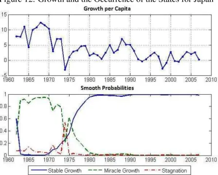
Figure 12 shows the regimes of Japan. In the 1960s and until the middle of the 1970s, the most
likely state is that of miraculous growth. After the oil shock growth decreased, stable growth continued.
This was followed by an exhaustion of the model of high savings and high investment surpluses, as Japan
already had the highest per capita GDP among the industrialized countries. There was a transition towards
an economy with more services and domestic consumption. Even during the “burst of the bubble” in 1989
and the early 1990s, the model does not place the country into a period of stagnation.
Figure 13 shows the growth pattern of the United States, which is similar to that of the countries that
were already industrialized in the beginning of the sample. Stable growth is the most likely state over the
entire period, with a small probability of stagnation and “catch-up” in the event of an oil shock.
Lastly, figure 14 shows the most probable states for the Congo, which is an African country with below
average institutions (-1.97). The stagnation state is predominant, with a possibility of stable growth during
the final years.
5
Conclusions and Extensions
In this study, we presented a model and estimation algorithm that allow for different growth states with
different linear sub-models, in the spirit of Pritchett (2003). The transition matrix depends on the
funda-mental characteristics of each country, which change over time. With this model, it is possible to examine
cur-rent works, and even to specialize in the study of growth in sub-models that are appropriate for diffecur-rent
circumstances.
In the empirical model, we further develop the first aspect, estimating a model where the
transi-tion depends on the quality of the institutransi-tions and on the level of investment. Three states were found,
where these coincide with the states identified by Pritchett (2003) and Jerzmanowski (2006). The role
of the institutions is critical in the dynamics of growth, and mainly influences the recuperation from
crises/stagnation and the stability of growth. The role of investment appears to be more restricted to
countries with good institutions, increasing the amount of time in the state of miraculous growth.
The evidence of the roles played by the quality of the institutions and by investment suggest strong
non-linearity and conditionality in the role of the explanatory variables, as indicated in various previous
studies, such as Kourtellos (2002), Tan (2010), and Jones and Olken (2008). The alternation between
states suggests that the series has many ruptures when analyzed by a linear framework, indicating the
need for more complex models for panel studies.
The estimated model also reinforces the evidence that the role of fixed effects cannot be disregarded,
even in a model for differences in growth. The level of the institutions (fixed for each country)
signifi-cantly influences growth, which is modeled in AR(1) for each state and which is equivalent to a differential
model, implying that the variation of growth in the estimated model is strongly conditioned by the level
of growth and by the fixed effects of the quality of the institutions.
The model that has been presented may be used as a more complex specification of the sub-models,
incorporating explanatory variables. We believe that this will be the most important sequence of this
work. New variables, such as per capita GDP, may be incorporated into the transition matrix, taking
care to maintain parsimony in the model. Eventually, with a change of the estimation algorithm, even
non-linear sub-models can be considered.
References
Aizenman, J. and Spiegel, M. (2007), Takeoffs, NBER Working Papers 13084, National Bureau of Economic
Research, Inc.
Alfo, M., Trovato, G. and Waldmann, R. J. (2008), “Testing for country heterogeneity in growth models using a
finite mixture approach”,Journal of Applied Econometrics, Vol. 23, pp. 487–514.
Ardic, O. P. (2006), “The gap between the rich and the poor: Patterns of heterogeneity in the cross-country data”,
Bai, J. and Perron, P. (2003), “Computation and analysis of multiple structural change models”,Journal of Applied
Econometrics, Vol. 18, pp. 1–22.
Basturk, N., Paap, R. and van Dijk, D. (2008), Structural differences in economic growth, Tinbergen Institute
Discussion Papers 08-085/4, Tinbergen Institute.
Bloom, D. E., Canning, D. and Sevilla, J. (2003), “Geography and poverty traps”,Journal of Economic Growth,
Vol. 8, pp. 355–78.
Breiman, L., Friedman, J., Olshen, R. and Stone, C. (1984),Classification and Regression Trees, Wadsworth and
Brooks, Monterey, CA.
Canova, F. (2004), “Testing for convergence clubs in income per capita: A predictive density approach”,
Interna-tional Economic Review, Vol. 45, pp. 49–77.
Dempster, A. P., Laird, N. M. and Rubin, D. B. (1977), “Maximum likelihood from incomplete data via the em
algorithm”,Journal of the Royal Statistical Society. Series B (Methodological), Vol. 39, Blackwell Publishing
for the Royal Statistical Society, pp. 1–38.
Desdoigts, A. (1999), “Patterns of economic development and the formation of clubs”,Journal of Economic Growth
, Vol. 4, pp. 305–30.
Diebold, F. X., Lee, J.-H. and Weinbach, G. C. (1993), Regime switching with time-varying transition probabilities,
Working Papers 93-12, Federal Reserve Bank of Philadelphia.
Durland, J. M. and McCurdy, T. (1994), “Duration-dependent transitions in a markov model of u.s. gnp growth”,
Journal of Business and Economic Statistics, Vol. 12, pp. 279–88.
Durlauf, S. N. and Johnson, P. A. (1995), “Multiple regimes and cross-country growth behaviour”, Journal of
Applied Econometrics, Vol. 10, pp. 365–84.
Easterly, W., Kremer, M., Pritchett, L. and Summers, L. H. (1993), “Good policy or good luck?: Country growth
performance and temporary shocks”,Journal of Monetary Economics, Vol. 32, pp. 459–483.
Filardo, A. J. (1994), “Business-cycle phases and their transitional dynamics”,Journal of Business and Economic
Statistics, Vol. 12, pp. 299–308.
Hall, R. E. and Jones, C. I. (1999), “Why do some countries produce so much more output per worker than others?”,
The Quarterly Journal of Economics, Vol. 114, pp. 83–116.
Hamilton, J. D. (1990), “Analysis of time series subject to changes in regime”,Journal of Econometrics, Vol. 45,
Hamilton, J. D. (1994),Time Series Analysis, 1 edn, Princeton University Press.
Hansen, B. E. (2000), “Sample splitting and threshold estimation”,Econometrica, Vol. 68, pp. 575–604.
Hausmann, R., Pritchett, L. and Rodrik, D. (2004), Growth accelerations, Working paper series, Harvard University,
John F. Kennedy School of Government.
Jerzmanowski, M. (2006), “Empirics of hills, plateaus, mountains and plains: A markov-switching approach to
growth”,Journal of Development Economics, Vol. 81, pp. 357–385.
Jones, B. F. and Olken, B. A. (2008), “The anatomy of start-stop growth”,The Review of Economics and Statistics
, Vol. 90, pp. 582–587.
Jong-A-Pin, R. and de Haan, J. (2007), Political regime change, economic reform and growth accelerations,
Tech-nical report.
Kerekes, M. (2009), “Growth miracles and failures in a markov switching classification model of growth”,Freie
Universitat Berlin, Discussion Papers, Vol. 11.
Knack, S. and Keefer, P. (1995), “Institutions and economic performance: Cross-country tests using alternative
institutional measures”,Economics and Politics, Vol. 7, pp. 207–227.
Kourtellos, A. (2002), A projection pursuit approach to cross country growth data, University of Cyprus Working
Papers in Economics 0213, University of Cyprus Department of Economics.
Loh, W.-Y. (2002), Regression trees with unbiased variable selection and interaction detection, Technical report,
Statistica Sinica.
Masanjala, W. H. and Papageorgiou, C. (2004), “The solow model with ces technology: nonlinearities and
param-eter hparam-eterogeneity”,Journal of Applied Econometrics, Vol. 19, pp. 171–201.
Paap, R., Franses, P. H. and van Dijk, D. (2005), “Does africa grow slower than asia, latin america and the middle
east? evidence from a new data-based classification method”, Journal of Development Economics , Vol. 77,
pp. 553–570.
Pritchett, L. (2000), “Understanding patterns of economic growth: Searching for hills among plateaus, mountains,
and plains”,World Bank Economic Review, Vol. 14, pp. 221–50.
Pritchett, L. (2003), A toy collection, a socialist star, and a democratic dud? growth theory, vietnam, and the
philippines.,in‘In Search of Prosperity: Analytical Narratives on Economic Growth. Princeton, NJ’, Princeton
Ruud, P. A. (1991), “Extensions of estimation methods using the em algorithm”,Journal of Econometrics, Vol. 49,
pp. 305–341.
Tan, C. M. (2010), “No one true path: uncovering the interplay between geography, institutions, and
fractionaliza-tion in economic development”,Journal of Applied Econometrics, Vol. 25, pp. 1100–1127.
Wacziarg, R. and Welch, K. H. (2003), Trade liberalization and growth: New evidence, Research papers, Stanford
University, Graduate School of Business.
Watson, M. (1983), “Alternative algorithms for the estimation of dynamic factor, mimic and varying coefficient