The Influence of Education on Economic Growth

(1)

243

The Influence of Education on Economic Growth

ŞTEFANăCRISTIANăCIUCU

RALUCA DRAGOESCU

Ph.D. Candidate

Cybernetics and Statistics Doctoral School,

The Bucharest University of Economics Studies

6ăPiațaăRoman ,ă1

st

District, Bucharest

ROMANIA

stefanciucu@yahoo.com; dragoescuraluca@gmail.com

Abstract

In transition countries affected by uncertainty, the educational system usually suffers from lack of funds from the government and it is affected by various reforms. It is important to see how education influences economic growth and how this growth can be improved by investing in education.

In this article, after a literature and econometric models review, the influence of primary, secondary and tertiary education over the GDP growth will be analyzed for Bulgaria, Czech Republic and the Netherlands, using regressions models, with the aid of computer software tool EViews. The models will be tested in order to obtain a good and reliable model.

Keywords: education, economic growth, GDP growth rate.

JEL classification: I25, C5.

1. Introduction

Education must be a priority for a proper development of a country. Education is a form of human capital, just like labor force, health, experience, training and other factors. The study of (Schultz, 1961) points out that both skills and knowledge that people gather during schooling years represent a form of human capital.

Economic growth in transition countries is a must in order to obtain an increase of the living standards of the people. From the economic growth, a part must always be invested in education, in order to achieve even higher growth.

Education is different in all the countries in the world and family and colleagues are important factors that contribute to education. Education also helps understand and process new information and implement new technologies (Hanushek, 2007).

(2)

244

2. Literature review

One of the main researchers on the role of education on economic output is Robert Barro. In (Barro, 1991) it is shown that human capital (as school enrollment rates) has a positive association with real GDP per Capita. In another work of (Barro, 1999), the schooling quality influence (using test scores) over economic growth is measured. Also, in (Barro, 1997), the contribution of education on economic growth is estimated, using the average years of attainment for males aged 25 and over in secondary and higher schools at the start of each period. In another work, (Barro and Sala-i-Martin, 1995) show that the average schooling years has a significant positive over the economic output.

Another interesting study is the one of (Bergerhoff, 2013), in which is raised the question about whether countries benefit from educating international students. The author proposes a model

andă usedă ită foră analysis.ă Theă modelă isă actuallyă aă “Solowă style”ă simplificationă ofă theă Lucasă modelă

(Lucas, 1988), that investigate the effects of internationalization in higher education on economic growth.

Khattak (2012), investigates the contribution of education to economic growth in Pakistan. In this study the Ordinary Least Squares (OLS) and Johansen Cointegration test as analytical techniques are used. The model is derived from an augmented form of Cobb Douglas Production Function, where real GDP per capita has been used as a measure for economic growth, physical capital is measured by gross fixed capital formation, secondary and elementary school enrollments have been used as measures for education and labor force participation rate for labor. The study shows that elementary as well secondary education contributes to Real GDP per Capita in Pakistan.

In the study of (Hanushek and Kimko, 2000) it is concluded that the results of mathematics and science in 31 countries are strong positively related to the growth of macroeconomic indicators. Education in Romania and Bulgaria is an interesting subject for researchers. For example the evolution of higher education in Romania during the transition period is analyzed in (Andrei, 2010) and a comparative study of some features of higher education in Romania and Bulgaria are done in (Andrei & Lefter, 2010).

3. Main models on the role of education over economic growth

The impact of education on economic growth has always been an interesting subject for economists and other specialists. There are many models that can be used for analyzing the impact of education on economic growth.

The starting point for many of these models is the following augmented form of Cobb Douglas Production Function:

(1) If human capital is introduced in equation (1), it becomes

(3)

245

In the study of (Mankiv, 1992), the MRW model is developed, in which the augmented Solow growth model solved for the steady-state per capita income level ends up to an equation that includes physical and human capital as the basic determinants of growth1.

The MRW model has employed a Cobb-Douglas production function of the following form (in which human capital is considered as an independent factor of production):

(3) The empirical form of the model can be written as:

(4) Linear models, LOG-LIN, LIN-LOG and LOG-LOG, can be used to describe the relationship between economic growth and education quantity and quality. First, in the LOG-LIN model (the dependent variable will be the logarithm of GDP growth, in our case), absolute change in the dependent variable will cause relative (percentage) change in the dependent variables. Second, in the LIN-LOG model, absolute change in the regressands is caused by relative (percentage) change in the dependent variable. Third, in the LOG-LOG model, relative change in the dependent variables will entail relative change in regressands.2

4. Methodology of the study

For the study, the multiple regression model used is:

The estimated multiple regression equation:

where:

= estimate of ; = estimate of ; = estimate of ; = GDP growth (%);

= gross enrolment ratio (primary, total)

= gross enrolment ratio, secondary (all programs, total) = gross enrolment ratio, ISCED 5 and 6 (total)

= random variable.

In order to obtain good estimates the least squares criterion will be used, choosing so as to (minimize the sum of square errors).

is the relationship between and , so if it is positive then that means that and are positively related and if it is negative then that means that they are negatively related.

1

Constantinos Tsamadias & Panagiotis Prontzas (2012): The effect of education on economic growth in Greece over the 1960–2000 period, Education Economics, 20:5, 522-537.

2

Akram Ochilov, Education and economic growth in Uzbekistan, Perspectives of Innovations, Economics & Business, Volume 12, Issue 3,

(4)

246

The multiple coefficient of determination , where SST = SSR + SSE.

The adjusted , noted .

The linear models, LIN-LIN, LOG-LIN, LIN-LOG and LOG-LOG for the multiple regression model will be tested, in order to obtain the best model.

5. Basic data interpretation

In this section, the data used in the study will be presented and briefly analyzed.

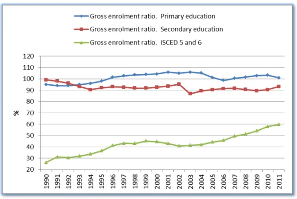
Figure 1. The evolution of gross enrolment ratio in Bulgaria Data source: UNESCO Institute for statistics

(5)

247

Figure 2. The evolution of the GDP growth rate in Bulgaria Data source: UNESCO Institute for statistics

Bulgaria has known a significant drop of the GDP after the political changes in 1989/1990 but the growth rate became positive from 1990 until 1996 when another steep decrease was recorded. After 1996 the GDP followed a similar evolution with other East European countries, being affected by the economic crisis in 2009.

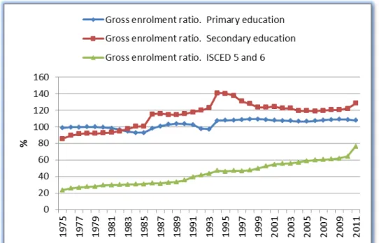
Figure 3. Gross enrolment ratio for primary, secondary and tertiary education for Czech Republic

(6)

248

While the gross enrolment ratio for primary and secondary education has slightly changed over the analyzed time horizon, the enrolment ratio for tertiary education recorded a constant increase in Czech Republic.

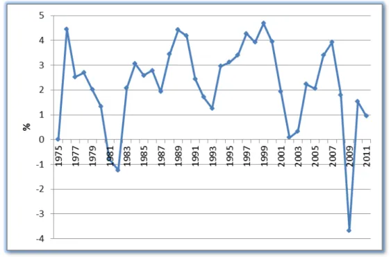
Figure 4. GDP growth ratio for Czech Republic Data source: UNESCO Institute for statistics

The GDP growth ratio for Czech Republic show a negative value in 1991 that was encountered for most of the ex-communist countries after the political changes in 1989 and then it starts to increase having positive but fluctuant values until 2009. The economic crisis resulted in a steep drop of the GDP growth ratio in 2009 followed by a relative recovery.

(7)

249

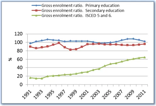
In The Nederlands the gross enrolment ratio for primary education has slightly increased over the analyzed time horizon while the gross enrolment ratio for tertiary education constantly increased. The gross enrolment ratio for secondary education increased until 1995 when it starts to decrease until 2010.

Figure 6. GDP growth ratio for Netherlands Data source: UNESCO Institute for statistics

Figure 6 shows that the GDP growth ratio for Nederlands dropped from 1976 to 1982. Between 1982 and 2008 the GDP growth ratio has fluctuated. There was an important drop in 2008 due to the economic crisis but the economy recovered and after 2008 the GDP growth ratio was positive.

6. Results and comments

A good regression model should have the following characteristics: a) a high R square value and a high adjusted R square value; b) most of the independent variables should be individually significant to explain dependent variable (can be tested using t-test); c) independent variables should be jointly significant to influence the dependent variable (f-test can be used); d) there should be no serial correlation in the residuals; e) the model should not have heteroskedasticity; f) residuals should be normally distributed. All these four features will be tested for our model.

The most important thing to be taken into consideration is that education quantity has an effect on economic growth after some years. The graduates have to start their career in order to affect the economy of a country. For this reason a time lag will be introduced in the model. The time lag for primary education will be set to 10 years and the time lag for secondary education to 5 years.

After testing the regression models for the three countries, the LOG-LIN model will be used.

c variable is the constant and primary_lag (primary education enrolment lagged by 10 years), secondary_lag (secondary education enrolment lagged by 5 years) and ISCED_5_6 (tertiary education enrolment, not lagged) are the independent variables. For each of the variables, the coefficient, standard error, t-statistics and p-value is displayed in the output.

(8)

250

Dependent Variable: LOG(GDP_G) Method: Least Squares

Date: 03/04/14 Time: 17:39 Sample: 2000 2011

Included observations: 11

Variable Coefficient Std. Error t-Statistic Prob.

C -6.391051 10.30228 -0.620353 0.5547

PRIMARY_LAG 0.202269 0.091535 2.209739 0.0628

SECONDARY_LAG -0.017522 0.087571 -0.200088 0.8471

ISCED_5_6 -0.224691 0.064962 -3.458829 0.0106

R-squared 0.720396 Mean dependent var 1.400947

Adjusted R-squared 0.600566 S.D. dependent var 0.856040

S.E. of regression 0.541024 Akaike info criterion 1.884582

Sum squared resid 2.048950 Schwarz criterion 2.029271

Log likelihood -6.365200 Hannan-Quinn criter. 1.793376

F-statistic 6.011806 Durbin-Watson stat 1.797327

Prob(F-statistic) 0.023794

Figure 7. Regression analysis output with all three independent variables for Bulgaria

The data included in the regression is from the 2000 to 2011 time period, because the main goal is to observe how education influences economic growth after the transition period started. Also, the data for primary education and secondary education was lagged by 10 respectively 5 years as previously stated.

The coefficient of determination is 0,720396, meaning that approximately 72,03% of the variability of the GDP growth is explained by the three education related variables.

Analyzing the Prob. column, which is actually the p-value, the least significant variable is the gross enrolment ratio in secondary education variable and the most significant variable is the gross enrolment ratio for tertiary education.

From the p-value of the F-statistics, it can be noticed that F-statistics is significant. This means that our three variables jointly influence the GDP growth in Bulgaria.

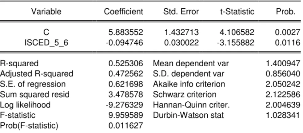
Students enrolled in tertiary education can be counted as labor force, so the following regression will be also commented:

Date: 06/04/14 Time: 09:11 Sample: 2000 2011

C 5.883552 1.432713 4.106582 0.0027

ISCED_5_6 -0.094746 0.030022 -3.155882 0.0116

(9)

251

The coefficient of determination is 0,525306, meaning that approximately 52,53% of the variability of the GDP growth is explained by ISCED_5_6 (tertiary education) variable. Also, the variable is individually significant to GDP growth and the model has a good f-statistic value, meaning that it is significant.

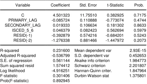
Next, the residuals distribution will be checked for the model in figure 7.

From figure 9, the Breusch-Godfrey serial correlation LM test (looking at the p-value), it can be noted that the residuals are not serial correlated, meaning that this model has not any serial correlations.

Breusch-Godfrey Serial Correlation LM Test:

F-statistic 0.753515 Prob. F(2,5) 0.5176

Obs*R-squared 2.547603 Prob. Chi-Square(2) 0.2798

Test Equation:

Dependent Variable: RESID Method: Least Squares Date: 06/04/14 Time: 09:40 Sample: 2000 2011

Presample and interior missing value lagged residuals set to zero.

C 4.501323 11.75510 0.382925 0.7175

PRIMARY_LAG -0.085724 0.110888 -0.773074 0.4744

SECONDARY_LAG 0.019333 0.106634 0.181302 0.8633

ISCED_5_6 0.046379 0.082423 0.562694 0.5979

RESID(-1) -0.392879 0.574216 -0.684201 0.5243

RESID(-2) -1.276338 0.881466 -1.447972 0.2073

R-squared 0.231600 Mean dependent var 2.93E-15

Adjusted R-squared -0.536799 S.D. dependent var 0.452653

Figure 9. The Breusch-Godfrey Serial Correlation LM test

For the heteroskedasticity test of the variance of the residuals, the Breusch-Pagan-Godfrey test has been used (figure 10). From the p-value of the test, it can be noticed that the residuals are homoscedastic.

Heteroskedasticity Test: Breusch-Pagan-Godfrey

Scaled explained SS 3.230005 Prob. Chi-Square(3) 0.3575

Test Equation:

Dependent Variable: RESID^2 Method: Least Squares Date: 06/04/14 Time: 09:44 Sample: 2000 2011

(10)

252

C 2.241608 4.127563 0.543083 0.6039

PRIMARY_LAG -0.051002 0.036673 -1.390724 0.2069

SECONDARY_LAG -0.000852 0.035085 -0.024297 0.9813

ISCED_5_6 0.064987 0.026027 2.496926 0.0412

Log likelihood 3.696257 Hannan-Quinn criter. -0.035980

Figure 10. Breusch-Pagan-Godfrey test

Finally, the residuals should be normally distributed. In order to check it, we used Jarque-Bera test. It can be noticed that the residuals are normally distributed (figure 11).

0 1 2 3 4

-1.25 -1.00 -0.75 -0.50 -0.25 0.00 0.25 0.50 0.75

Series: Residuals Sample 2000 2011 Observations 11

Mean 2.93e-15

Median -0.000710

Maximum 0.577281

Minimum -1.010772

Std. Dev. 0.452653 Skewness -0.784086 Kurtosis 3.311958

Jarque-Bera 1.171719 Probability 0.556627

Figure 11. Jarque-Bera test

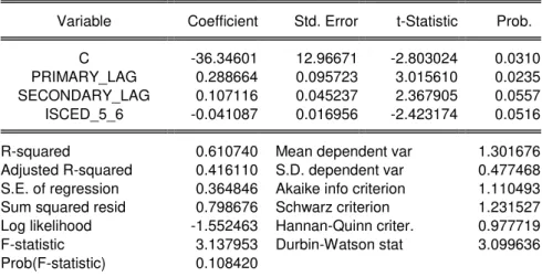
 The regression model estimations for the Czech Republic are presented below:

Date: 03/04/14 Time: 17:35 Sample: 2001 2011

C -36.34601 12.96671 -2.803024 0.0310

PRIMARY_LAG 0.288664 0.095723 3.015610 0.0235

SECONDARY_LAG 0.107116 0.045237 2.367905 0.0557

ISCED_5_6 -0.041087 0.016956 -2.423174 0.0516

(11)

253

The data included in the regression are from the 2001 to 2011 time period, because the main goal is to observe how education influences economic growth after the transition period started. The data were lagged by 10 respectively 5 years as for Bulgaria.

The R-squared value is approximately 61,07%. This means that 61% of the variability of the GDP growth is explained by the three education related variables.

As in the case of Bulgaria, in order to have a good regression model most of the independent variables should be individually significant to influence the GDP growth. As seen from the Prob. column, the most significant variable is the gross enrolment ratio for primary education. The other two variables are at the limit of being significant or not.

The F-statistics value of the model, from which we can determine the jointly significance of the variables to explain the dependent variable is high meaning that the variables are not so good at explaining the GDP growth.

Running the Breusch-Godfrey Serial Correlation LM test, it can be observed that the residuals are not serial correlated, meaning that this model has not any serial correlations.

From the Breusch-Pagan-Godfrey test, it can be stated that the residuals have a constant variance, meaning that residuals are homoscedastic, which is a good feature for the model.

The last test, the Jarque-Bera test, is used to check if the residuals are normally distributed. The Jarque-Berra statistics is 0.590287 and the corresponding p value is 0.744425 (74,44%), meaning that population residual is normally distributed.

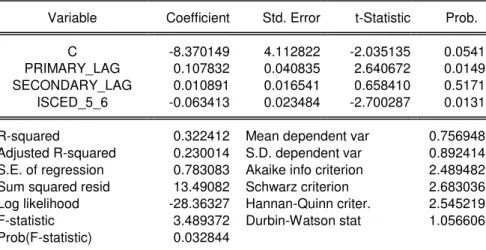
 The regression model estimates for the Netherlands are presented below:

Date: 03/04/14 Time: 18:14 Sample: 1985 2011

C -8.370149 4.112822 -2.035135 0.0541

PRIMARY_LAG 0.107832 0.040835 2.640672 0.0149

SECONDARY_LAG 0.010891 0.016541 0.658410 0.5171

ISCED_5_6 -0.063413 0.023484 -2.700287 0.0131

Figure 13. Regression analysis output with all three independent variables for the Netherlands

The data included in the regression are from the 1985 to 2011. The data were also lagged by 10 respectively 5 years as previously stated.

The R-squared value is less than in Bulgaria and Czech Republic case, 0.322412, meaning that only 32,24% of the variability of the GDP growth is explained by the three education related variables. Instead, the variables are more individually significant in the Netherlands case than

inăBulgariaăorăCzechăRepublic’săcase.ăAlso,ăfromătheăf-statistics it can be observed that overall the

independentăvariablesăareăjointlyăsignificantătoăinfluenceătheăGDPăgrowthăjustălikeăinăBulgaria’săcase. LikeăinăBulgaria’săcase,ăstudentsăenrolledăinătertiaryăeducationăcanăbeăcountedăasălaborăforce,ăsoătheă

(12)

254

Dependent Variable: GDP_G Method: Least Squares Date: 04/08/14 Time: 15:12 Sample: 1985 2011

C 5.311499 1.360007 3.905493 0.0006

ISCED_5_6 -0.058862 0.027028 -2.177827 0.0391

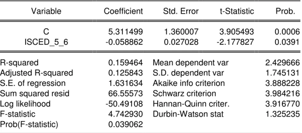
Figure 14. Regression output only with ISCED_5_6 as independent variable for the Netherlands

In the Netherlands only 15,94% of the variability of the GDP growth is explained by

ISCED_5_6 (tertiary education) variable. The p-value of the variable is good, meaning that it is significant at a level of 5%. Also, from the f-statistics it can be noted that the model is significant.

Running the Breusch-Godfrey serial correlation LM test for the model in figure 13, we obtain:

Breusch-Godfrey Serial Correlation LM Test:

Test Equation:

Dependent Variable: RESID Method: Least Squares Date: 04/08/14 Time: 15:17 Sample: 1985 2011

Presample and interior missing value lagged residuals set to zero.

C 1.750998 3.792150 0.461743 0.6492

PRIMARY_LAG -0.016335 0.038439 -0.424943 0.6754

SECONDARY_LAG -0.004232 0.015519 -0.272677 0.7879

ISCED_5_6 0.008125 0.021351 0.380564 0.7075

RESID(-1) 0.595496 0.227987 2.611975 0.0167

RESID(-2) -0.193144 0.245171 -0.787794 0.4401

R-squared 0.267400 Mean dependent var 7.81E-16

(13)

255

From the test in figure 15, it can be observed that the residuals of this model are serially correlated.

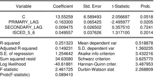
Next the Breusch-Pagan-Godfrey test will be run in order to determine if the variance of the residual is homoscedastic or heteroscedastic.

Heteroskedasticity Test: Breusch-Pagan-Godfrey

Scaled explained SS 15.45750 Prob. Chi-Square(3) 0.0015

Test Equation:

Dependent Variable: RESID^2 Method: Least Squares Date: 04/08/14 Time: 15:18 Sample: 1985 2011

C 13.55259 6.589493 2.056697 0.0518

PRIMARY_LAG -0.163300 0.065425 -2.495977 0.0205

SECONDARY_LAG 0.009475 0.026502 0.357510 0.7241

ISCED_5_6 0.049557 0.037626 1.317100 0.2014

Figure 16. Breusch-Pagan-Godfrey test for the Netherlands model

Looking at the output from figure 16, it can be seen that the variance of the residual is homoscedastic.

Using the Jarque-Berra statistics, it can be determined whether the residuals follow a normal distribution or not.

0 2 4 6 8 10 12

-3.0 -2.5 -2.0 -1.5 -1.0 -0.5 0.0 0.5 1.0 1.5

Series: Residuals Sample 1985 2011 Observations 26

Mean 7.81e-16

Median -0.062811

Maximum 1.192710

Minimum -2.624415

Std. Dev. 0.734597 Skewness -1.590617 Kurtosis 7.607920

Jarque-Bera 33.96593 Probability 0.000000

(14)

256

From the output of figure 17 we can conclude that the residuals are not normally distributed.

7. Conclusions

In this article, after searching and testing several models, three LOG-LIN models are proposed. After testing each of the models it can be observed that all of them have both strengths and weaknesses.

The main point that is demonstrated is that education has an influence on economic growth in both transition and developed countries. The level of influence varies and depends on other factors from country to country.

What is interesting to observe is that a negative relationship exists between GDP growth and tertiary education in all three countries. A very good explanation about this phenomenon is provided in (Ochilov, 2012) and just like in Uzbekistan case, in all three countries (Bulgaria, Czech Republic and the Netherlands) tertiary schools educate and re-educate existing workers, meaning that actually instead of working and contributing to GDP growth, people are going to tertiary schools. Also, high educated persons demand higher wages.

Taking a look at all three models it can be observed that the secondary enrolment variable is the least significant variable of the three independent variables.

The best regression model can be considered the one for Bulgaria, because two out of three independent variables are significant and the variables jointly influence GDP growth. Also, the model has not any serial correlation and the residuals are homoscedastic. Another important thing is that from Jarque-Berra test population residual is normally distributed.

Due to the fact that few data are used, it can be consider that a calibration of each of the models has been obtained. As further development of the study, a panel data regression model is suitable.

References:

1. Schultz, T.W., (1961), "Investments in human capital", American Economic Review 51:1–1.7 2. Hanushek,ăE.ă&ăWöβmann,ăL.,ă(2007),ă„TheăRoleăofăEducationăQualityăinăEconomicăGrowth”,ă

World Bank PolicyResearch Working Paper 4122.

3. Mankiw,ăG.,ăRomer,ăD.,ă&ăWeil,ăD.,ă(1992),ă“AăContributionătoătheăEmpiricsăofăEconomică

Growth.ăTheăQuarterlyăJournalăofăEconomics”,ăno.ă2,ăpp.ă407-437.

4. Barro,ăR,ăJ.,ă(1991),ă“EconomicăGrowthăinăCross-SectionăofăCountries”,ăTheăQuarterlyăJournală of Economics, Vol.106, No.2, pp.407-443.

5. Barro,ă R.,ă (1997),ă “Determinantsă ofă economică growth:ă Aă cross-countryă empiricală study”,ă Cambridge, MA: MIT press.

6. Barro, R., (1999),ă “Humană Capitală andă Growthă ină Crossă Countryă Regressions,”ă Swedishă Economic Policy Review, Vol.6, pp.237-77.

7. Barro, R., Sala-i-Martin, X., (1995), Economic Growth, McGraw-Hill, New York.

8. Hanushek, E., Kimko, D. , (2000), "Schooling , labour force quality and the growth of nations", American Economic Review 90, No 5: 1184-1208.

9. Bergerhoff,ăJ.,ăBorghans,ăL.,ăSeegers,ăP.,ăvanăVeen,ăT.,ă(2013),ă“InternationalăEducationăandă

EconomicăGrowth”,ăDiscussionăPaperăNo.ă7354,ăIZA.

10. Lucas,ă E.,ă (1988),ă “Onă theă Mechanicsă ofă Economică Development”,ă Journală ofă Monetaryă Economics, no. 22, 342.

11. Khattak,ăNaeemă UrăRehman,ăKhan,ăJ.,ă(2012),ă“Theăcontributionăofăeducationătoăeconomică

growth:ăevidenceăfromăPakistan”,ăInternationalăJournalăofăBusinessăandăSocialăScienceă,ăVol.ă

3, No. 4: pp. 145-151.

12. Andrei,ăT.,ăTeodorescu,ăD.,ăOancea,ăB.,ăIacob,ăA.,ă(2010),ă“Evolutionăofăhigherăeducationăină

(15)

257

13. Andrei, T., Lefter, V., Oancea, B., Stancu, S., (2010),ă“Aăcomparativeăstudyăofăsomeăfeaturesă

ofă higheră educationă ină Romania,ă Bulgariaă andă Hungary”,ă Romaniană Journală ofă Economică

Forecasting – Volume 13, Issue 2, pp. 280-294.