Working
Paper
397
Forecast Comparison With Nonlinear
Methods For Brazilian Industrial
Production
Jordano Vieira Rocha
Pedro L. Valls Pereira
CEQEF - Nº24
Working Paper Series
WORKING PAPER 397–CEQEF Nº 24•JULHO DE 2015• 1
Os artigos dos Textos para Discussão da Escola de Economia de São Paulo da Fundação Getulio Vargas são de inteira responsabilidade dos autores e não refletem necessariamente a opinião da
FGV-EESP. É permitida a reprodução total ou parcial dos artigos, desde que creditada a fonte.
FORECAST COMPARISON WITH NONLINEAR
METHODS FOR BRAZILIAN INDUSTRIAL
PRODUCTION
∗
Jordano Vieira Rocha
Sao Paulo School of Economics - FGV and CEQEF - FGV
Pedro L. Valls Pereira
Sao Paulo School of Economics - FGV and CEQEF - FGV
Abstract
This work assesses the forecasts of three nonlinear methods — Markov Switching Autoregressive Model, Logistic Smooth Transition Autoregressive Model, and Auto-metrics with Dummy Saturation — for the Brazilian monthly industrial production and tests if they are more accurate than those of naive predictors such as the autore-gressive model of order p and the double differencing device. The results show that the step dummy saturation and the logistic smooth transition autoregressive can be superior to the double differencing device, but the linear autoregressive model is more accurate than all the other methods analyzed.
Keywords: Forecasting; Nonlinear methods; Markov Switching; Smooth Trans-ition Autoregressive; Autometrics; Dummy Saturation.
1
Introduction
Classic econometric models assume a number of restrictive hypotheses about the included random variables. These hypotheses are made in general to simplify the model, but are later relaxed. In this context, time series based modeling does not depart from the pattern.
Some assumptions, however, many made implicitly, are not relaxed. It is supposed that economic time series are realizations of stochastic processes, represented by a Data Generating Process, denoted henceforth DGP1. The DGP, in turn, has its form known, and is assumed
fixed in the sample period.
∗Second author received financial support from CNPq and FAPESP. 1
However, econometric models forecasts under the hypothesis of structural breaks have been gaining more attention in the last years specially after the subprime financial crisis. The abrupt changes in the dynamic of several economic and financial series have caused a phenomenon called forecast failure by David Hendry,i.e., persistent failures in the forecasts after a certain period. In a world that, as it is becoming more evident, is not stationary, subject to structural breaks, and nonlinear, traditional modeling techniques are discovered to be ineffective to the economic process’ comprehension and, mainly, to variable prediction. Having this in mind, it is a valid exercise to try to define robust forecasting mechanisms. Hendry (2006) suggests that to predict using the difference of a series (even a stationary one) would make its forecast robust. In the moment of a structural break occurrence, the forecast would be biased, since this change would be unpredictable. In the following periods, however, the forecast would become unbiased, correcting the forecast failure.
Another option — that is useful for both in-sample modeling and forecasting — is to use different econometric techniques that account for those characteristics that better capture the nonlinear behavior of some economic variables. Many nonlinear models already exist in the literature. Many of the most notable are composed by a set of linear models that alternate between them in time according to some rule of transition. It is the case of the Smooth Transition Autoregressive Model (STAR) and the Markov Switching Autoregressive (MSAR). The former has the changing rule based in a transition function and the latter based in a probabilistic structure. STAR transitions are more abrupt than those of MSAR, because, in the latter, the transitions are ruled by a Markov Process. This process is characterized by a transition matrix which give the probabilities of switching between regimes, and this characterizes the smoothness of transitions.
Another form of capturing nonlinearities is through the introduction of dummies that detect outliers and level shifts. A methodology proceeding this way is described by Doornik (2009). This technique consists in an automatic variable selection method. Thereby, the change in the series’ mean would be modeled by the automatic selection of step and impulse dummies, modifying the conditional mean and avoiding repeatedly wrong forecasts which would tend to be biased towards the previous unconditional mean.
Some works have been made with the objective of modeling many economic variables according with the nonlinear techniques. In the case of STAR models, for example, Ter¨asvirta (1992) analyze the evolution of quarter industrial production indexes from several countries. As examples of works using Markov Switching, we can cite Engel (1994), who models the US dollar exchange rate.
The literature involving automatic variable selection and Dummy Saturation is more scarce, as its theory was developed recently and its practical implementation with the eco-nometric package Oxmetrics is even more recent. Examples of applications can be found in Hendry & Mizon (2011) who analyze the expenditure in food in United States.
2
Theoretical Review
This section is based in Hendry (2012), which simplifies the more general theory with multiple variables in Hendry (2006).
Consider a variable yt that we want to predict. Suppose yt ∼ Dyt(yt|Yt−1, θ), where
θ ∈ Θ ⊆ Rk and Y
t−1 = (y1, . . . , yt−1). For a sample of size T, a forecast h step ahead
is a combination of the sample values from 1 through T, i.e., ˆyT+h|T = fh(YT). It can be proven (for example in Clements & Hendry (1998)) thatyT+h|T =E[yT+h|YT] is the unbiased predictor which minimizes the Mean Square Forecast Error (MSFE) and holds the minimum variance within the unbiased predictor class.
Suppose yt follows the linear autoregressive process below:
yt =µ+ρyt−1 +γzt+ǫt, with ǫt∼IN(0, σǫ2) e |ρ|<1 (1) where {zt} is an exogenous variable, forecast error’s mean and variance are, respectively,
E[yT+1−yT+h|T] = 0 and V[(yT+1−yT+h|T)] =σǫ2.
Consider E[yt] =θ and zt ∼N(κ,1). We can write the mean of yt as:
E[yt] =θ= µ+γκ
1−ρ (2)
Ifµ=κ= 0, a break inρwill not affect the mean ofyt. However, in case that we have one of these parameters different from zero, a change in the autoregressive parameter will imply a change in the mean. Besides this, if more than one of these parameters suffer a break, the forecast failure can be even more severe. For example, if the autoregressive parameter and the intercept, ρ and µ, are, respectively, 0.8 and 8, and suffer a break, becoming 0.6 and 6, the unconditional expectation shifts from θ= 40 to θ∗ = 15.
Let us rewrite the model (1) as:
∆yt=µ+ (ρ−1)yt−1+γzt+ǫt+ (ρ−1)
µ+γκ
1−ρ −(ρ−1)
µ+γκ
1−ρ
!
=µ−µ−γκ+ (ρ−1)(yt−1−θ) +γzt+ǫt = (ρ−1)(yt−1−θ) +γ(zt−κ) +ǫt
The forecasts i steps ahead are given by:
∆yT+i =ω+α(yT+i−1−θ) +γzT+i+ǫT+i (3) whereω =−γκ and α=ρ−1.
This formulation is denoted Equilibrium Correction Model (EqCM), where the equilib-rium is given by θ. Forecasts will tend to return to θ independently of the behavior of the data. Changes in this equilibrium, which occur mainly by shifts in the level, consist in the main factor which imply forecast failure.
second differences have unconditional expectationE[∆2xt] = 0, suggesting the following DDD
estimator:
f
∆yT+1|T = ∆yT (4)
where∆fyT+1|T denotes a one-step ahead forecast for ∆yT given the information in timeT. Because the forecast does not utilizes any parameter, structural breaks do not persistently influence it, and the estimator is unbiased.
Let us modify equation (3) so that the DGP does not contain exogenous variables besides the dependent variable lags (i.e. γ = 0):
∆yT+i =α(yT+i−1−θ) +ǫT+i (5) Suppose there is a break in the parameters, so that the DGP becomes:
∆yT+i =α∗(yT+i−1−θ∗) +ǫT+i (6) EqCM forecast error is given by:
∆yT+i−∆cyT+i|T+i−1 = ∆yT+i−αˆ(yT+i−1−θˆ) +ǫT+i =wT+i (7) where the hat over the parameters means that they were estimated on the EqCM formulation. Replacing the in-sample estimated values for the pseudo-true in-sample population values, where E[ˆθ] = θp, we can reduce the forecast error variance without damage to the general analysis. Thus, we have:
E[wT+i|yT+i−1] = (α∗θ∗−αpθp) + (α∗−αp)yT+i−1
VT+i[wT+i|yT+i−1] =σǫ2 (8)
With respect to the DDD (∆fyT+i|T+i−1 = ∆yT+i−1), for i >1, we have:
∆yT+i−1 =α∗(yT+i−2−θ∗) +ǫT+i−1 (9)
The respective forecast error is calculated as:
∆yT+i−∆fyT+i|T+i−1 =uT+i =α∗(yT+i−1−θ∗) +ǫT+i −[α∗(y
T+i−2−θ∗) +ǫT+i−1] (10)
⇒uT+i =α∗∆yT+i−1+ ∆ǫT+i (11)
On the long term, values are replaced by their unconditional expectations, i.e.:
E[uT+i] =α∗E[∆yT+i−1] +E[∆ǫT+i] = 0 (12) V[uT+i] =V[α∗∆yT+i−1] +V[∆ǫT+i]
As it is evident from (11) and (13), the Double Differencing mechanism adds some noise sources by the extra differentiation of α∗y
T−i+1 and of ǫT+i. This extra source of noise,
however, can be of lower dimension than those from the traditional autoregressive model when there is presence of structural breaks in the series’ unconditional mean.
To illustrate, suppose that the shift occurs only in µ, so that θ changes and α remains constant. We will have:
wT+i =−α(θ∗−θ) +ǫT+i
E[wT+i] =−α(θ∗−θ) V[wT+i] =σǫ2
uT+i =α∆yT+i−1+ ∆ǫT+i
E[uT+i] = 0
V[uT+i] =V[α∆yT+i−1] +V[∆ǫT+i]
The MSFE is approximately:
M[wT+i] =α2(θ∗−θ)2+σǫ2 (14)
Comparing with the DDD MSFE:
M[uT+i] = 2σǫ2 1 +
α2
2 +α
!
(15)
Assuming ρ = 0.8, ∇µ∗ = µ∗ −µ = 0.2, and σ
ǫ = 0.06, we have α = −0.2 and ∇θ∗ =
θ∗−θ = 1. With these values,M[w
T+i] is approximately 6-fold larger than M[uT+i].
To avoid the forecast failure problem, it is also possible to use nonlinear modeling methods which are able to detect a change in the series behavior. Next section we will review the methodology of three nonlinear models’ that are used on this work.
2.1
Markov Switching Autoregressive Model (MSAR)
This technique supposes that the DGP consists in different autoregressive models which alternate between them according to a process represented by a discrete latent variablest= {1,2, . . . , N}, in which each value represents a different regime. An additional assumption is that st follows a Markov process, i.e., the probability of the realization of state j in the current period depends only of the realization of the state from the immediately previous period:
P =
p11 p21 . . . pN1
p12 p22 . . . pN2
... ... ... ...
p1N p2N . . . pN N
(17)
Suppose, for simplicity and without loss of generality, an AR(1) process in which the intercept and autoregressive values change according to each regime. We can write this process as:
yt=cst +φstyt−1+εt (18)
where we assume that εt∼i.i.d.N(0, σ2) and is independent of st.2
Observe that, even if we know all the involved parameters, we cannot affirm certainly in which regime the process is in each period. We infer the state, conditional to the realization of the series values up to T, by P(st = j|yt, θ), given, following the law of conditional probabilities, by:
P(st=j|yt, θ) =
p(yt, st =j, θ)
f(yt, θ)
= πjf(yt|st =j, θ)
f(yt, θ)
(19)
In the expression above, πj =P(st=j, θ) is the unconditional probability ofst assuming the valuej, f(yt|st=j, θ) is the conditional density, assumed normal, that is:
f(yt|st=j, θ) = 1 √
2πσj
expn−(yt−cst −φstyt−1)
2
2σ2
j
o
(20)
and the unconditional density is given by:
f(yt, θ) = N X
j=1
p(yt, st =j, θ) = N X
j=1 πj √
2πσj
expn−(yt−cst−φstyt−1)
2
2σ2
j
o
(21)
Stacking the conditional densities f(yt|st = j, θ), the conditional probabilities P(st =
j|yt, θ) and the forecasts P(st+1 =j|yt, θ) in vectors (N×1), respectively, ηt, ˆξt|te ˆξt+1|t,i.e.,
2
In general, the variance of the error term also depends on the underlying regime,i.e.,εs
t ∼i.i.d.N(0, σ
2
st).
ηt=
f(yt|st = 1, yt−1;θ) f(yt|st = 2, yt−1;θ)
...
f(yt|st =N, yt−1;θ)
(22) ˆ
ξt|t=
P(st = 1|yt, θ)
P(st = 2|yt, θ) ...
P(st=N|yt, θ) (23) ˆ
ξt+1|t=
P(st+1 = 1|yt, θ)
P(st+1 = 2|yt, θ) ...
P(st+1 =N|yt, θ)
(24)
Hamilton (1994) shows that the optimal inference for the regimes is given by the following recursion:
ˆ
ξt|t=
( ˆξt|t−1⊙ηt)
1′( ˆξ
t|t−1⊙ηt)
(25)
ˆ
ξt+1|t=Pξˆt|t (26)
where⊙ represents element-by-element multiplication and 1 is a vector (N ×1) of 1’s. The log-likelihood maximization problem is given, thus, by:
max L(θ) = T X
t=1
f(yt|yt−1, θ) =
T X
t=1
1′( ˆξt|t−1⊙ηt) (27)
s.t. (pi1 +pi2+· · ·+piN) = 1, pij ≥0,∀j, i (28) The expression (25) is analogous to (19), and (27), analogous to (21).
Given the values of θ0 and ˆξ1|0 (e.g. ξˆ1|0 = ρ, with ρ = 1/N), the recursion in (25)-(26)
returns the values of ˆξt|t. Note that, for eacht, this method utilizes only the realized values in
the current and in previous periods (t, t−1, t−2, . . .) in order to estimate P(st =j|yt−1, θ).
However, we possess additional information to increase this estimate’s accuracy, namely, the remainder of the sample (t+ 1, t+ 2, . . . , T). For this, we have to use a smoothed inference mechanism.
Let us denote, generalizing the previous notation, the probability of being in a regime conditional to the realized values from the series and to the parametersP(st =j|yτ, θ). For
t < τ, we will have a smoothed inference of regime t. Kim (1994) develops a recursion
analogous to (26):
ˆ
ξt|T = ˆξt|t⊙
where (÷) means term-by-term division.
The iteration algorithm starts in ˆξT|T, which, in turn, is calculated from (25)-(26), passing through ˆξT−1|T,ξˆT−2|T, . . . ,ξ1ˆ|T. Once having ˆξt|tand ˆξt+1|tknown,θ is obtained solving (27)-(28), proceeding recursively until there is convergence to aθ∗. Hamilton (1990) demonstrate
the the transition probabilities estimators pij are given by:
ˆ
pij = PT
t=2P(st=j, st−1 =i|yT, θ) PT
t=2P(st−1 =i|yT, θ)
(30)
that is the sum of the probabilities of regimeibeing followed by regimej divided by the sum of the probabilities of being in regime i.
Finally, to calculate the optimal forecast one-step ahead, suppose we know which will be the regime in periodt+1, so the prediction will be obtained byhjt =E(yt+1|st+1 =j,Yt;θ) = R
yt+1f(yt+1|st+1 = j,Yt;θ)dyt+1, where Y is a vector containing all y observations through
date t. The unconditional expectation will be, thus, given by:
E(yt+1|xt+1,Yt;θ) = Z
yt+1f(yt+1|xt+1,Yt;θ)dyt+1
= Z
yt+1
nXN
j=1
p(yt+1, st+1 =j|xt+1,Yt;θ) o
dyt+1
= Z
yt+1
nXN
j=1
[f(yt+1|st+1 =j, xt+1,Yt;θ)P(st+1 =j|xt+1,Yt;θ)] o
dyt+1
= N X
j=1
P(st+1 =j|xt+1,Yt;θ) Z
yt+1f(yt+1|st+1 =j, xt+1,Yt;θ)dyt+1
= N X
j=1
P(st+1 =j|Yt;θ)E(yt+1|st+1 =j, xt+1,Yt;θ) (31)
If we stackhjt in a vector (N ×1)ht, then:
E(yt+1|Yt;θ) =h′tξt+1|t (32)
Although the Markov Chain admits a linear representation, the optimal forecast one-step ahead is a nonlinear function of the of the observed variables, for ξt|t depends on Yt in a nonlinear way. This implies that, if, inside a regime, it is observed an outlier, that is, an observation little likely to be generated in this regime, the framework analyzed here has high probability of inferring that a change of state has occurred.
2.2
Smooth Transition Autoregressive Model (STAR)
Suppose a stochastic process represented by the following DGP:
yt=π10+π1′zt+ (π20+π2′zt)F(yt−d) +ǫt (33)
F(yt−d) is called the transition function, it depends on the model’s dependent variable,
yt, lagged by the parameter d, that will be estimated. The vector zt = (yt−1, yt−2, . . . , yt−p) contains the lagged series, (π1, π2) are parameter vectors with correspondent dimensions and
(π10, π20) are scalars. The error term is assumed normal, independent and identically
distrib-uted,i.e.,ǫt ∼i.i.d.N(0, σ2). It is important to stress that ǫtis symmetric, so that rejections of the null hypothesis from linearity tests would come from the model parametrization, and not from the error term.
The F function is limited between 0 and 1. In case it is an indicator functionF(yt−d) =
I(yt−d> c)3, the model is denotedSelf Exciting Threshold Autoregressive(SETAR), in which, whenyt−dis greater than the thresholdc, the regime is changed instantaneously. To establish a smooth transition between the regimes, we can use some continuous function between 0 and 1, so that the parameters of (33) vary, as function of yt−d, between π10 and (π10+π20)
for the intercept, and between π1 and (π1 +π2), for the autoregressive parameters. These values correspond to the two extreme regimes (F = 0 andF = 1, respectively).
There are two functions used predominantly in the literature. The first is the logistic function:
F(yt−d) = (1 +exp[−γ(yt−d−c)])−1 (34) When the model uses the function above, it is calledLogistic Smooth Transition
Autore-gressive (LSTAR). The inclination parameter γ measures the speed of transition from one
regime to another, and the location parametercis the threshold. Besides, whenγ → ∞, the model approximates a SETAR model.
LSTAR model has been used to model macroeconomic series with asymmetric behavior. ¨
Ocal & Osborne (2000) and Ter¨asvisrta & Anderson (1992) use it to model industrial pro-duction series and Skalin & Ter¨asvirta (2002) for unemployment series.
The second function is the exponential function:
F(yt−d) = 1−exp(−γ(yt−d−c)2) (35) Using this function, we denote the model Exponential Smooth Transition Autoregressive (ESTAR). The interpretation given to the parameters γ and c is the same as in LSTAR. When γ → ∞, however, F tends to I(yt−d=c).
The ESTAR model is normally utilized in series with symmetric behavior. In this case, we would have one regime when yt−d gets near the threshold and another when it gets far. An example of application is Arango & Gonzalez (2001), who models the Colombian inflation acceleration.
To verify if there are gains in formulating a nonlinear specification, we should do a linearity test. Besides, we will need this test to estimate the parameterd. There is, however, a caveat in performing this test, for there are many ways of defining linearity in (33)-(34)/(35).
3
We will use, in this work, only two regimes, corresponding in theory to periods of expansion and periods of recession, but we could generalize for more regimes. In this case, the model would have, in the indicator function example, the formyt=P
r
When we test H01 : γ = 0 in (33)-(34), the model will be identified only under the alternative hypothesis, becauseπ20 and π2 will be able to assume any value. If, on the other side, we testH01:π20, π2 = 0, γ and cwill be able to assume any value. A similar reasoning
applies to (33)-(35).
To contour this problem, Ter¨asvirta (1994), based on Davies (1977) and on Luukkonen et al. (1988) elaborates a test from a Taylor expansion around γ = 0, leading to the following auxiliary regression:
ˆ
ut = ˆw′1tβ1˜ + p X
j=1
β2jyy−jyt−d+ p X
j=1
β3jyy−jy2t−d+ p X
j=1
β4jyy−jyt3−d+v′t (36)
where ˆut are the residuals from the (linear) AR(p) model estimation, ˆw1′t = −(1, zt′)′ and ˜
β1 = (β10, β1′)′. The null hypothesis of linearity is:
H0′ :β2j =β3j =β4j = 0, j = 1, . . . , p (37)
Each βij is a combination of the parameters from (33), different, thus, for (34) and (35). Comparing these combinations, (36) will have different formats and Ter¨asvirta (1994) elaborates successive F-tests which can distinguish between on function and another. They are4:
1. H′
01:β4 = 0.
2. H′
02:β3 = 0|β4 = 0.
3. H′
03:β2 = 0|β3 =β4 = 0.
If H′
01 is rejected, we have evidence in favor of the LSTAR model, otherwise, we can use
the ESTAR model. If H′
10 and H20′ are accepted, we also have evidence in favor of LSTAR,
the hypothesis rejection, however, is nor informative. If the true model is a LSTAR, H′
03 is
generally rejected. If H′
03 is accepted and H02′ is rejected, we choose the ESTAR model. If H′
03and H02′ are accepted, butH01′ rejected, LSTAR model is selected. The only inconclusive
case is whenH′
01 and H02′ are rejected. In this situation, we test:
H02′′ :β3 = 0|β2 =β4 = 0 (38)
However, if H′
02 is rejected, H02′′ should be rejected even more strongly.
Parameter estimation can be done by Nonlinear Least Squares, that, under the assumption of normality, is equivalent to the estimation of Conditional Maximum Likelihood. Under some assumptions and regularity conditions (Wooldridge, 1994), estimators are consistent and asymptotically normal. The estimation procedure is thus carried out with standard numerical algorithms (e.g. Newton-Raphson and BFGS).
This work’s objective is to make one-step ahead forecasts, re-specifying the model at each period. It is, therefore, impracticable and counter-intuitive to decide, at each step, if
4
The notation βi = 0|βj = 0 means that the testβi = 0 is made conditional on the non-rejection of the
previous testβj= 0. Thus,H02′ is made conditional on the non-rejection ofH01′ , andH03′ is made conditional
on the non-rejection ofH′
the DGP comes from a STAR model with logistic function or with an exponential function. Impracticable for the fact that the test explained above for the most appropriate function contains inconclusive situations, making it difficult to construct an algorithm for real-time automatic forecast. Counter-intuitive because the change in the function at each step would imply that, given the information at each new observation, the entire series generating process would be revalued, being governed alternatively by a function characterizing asymmetric series and by a function characterizing symmetric series.
As the series to be analyzed here (Brazilian industrial production, as will be explained ahead with more details) has an asymmetric behavior, i.e., it grows more slowly than it decreases, we opted to use only the logistic function in the specification of the STAR model. Castle & Hendry (2013) investigate, through Monte Carlo simulations, the LSTAR models forecast and estimation efficiency for different magnitudes in the transition probability from one regime to another and differences between the intercepts of each regime. They conclude that, for very highγ’s, estimation becomes imprecise. Besides, there must be a large number of observations in each regime. For this to happen in small samples, it would be necessary a large probability of change between regimes. On the other side, the constant change of regimes can imply that the series is better modeled by a linear autoregressive process. These problems tend to be solved in reasonably large samples, as it is the case of this work.
Concerning the forecast results, estimation precision, measured by the Root Mean Squared Forecast Error (RMSFE), of a correctly specified LSTAR with one lag is superior in large samples and when the difference in the mean of each regime is not very large nor vert small (the cited authors analyze changes of 1, 2, and 5 standard-deviations in the intercept).
From equation (33), the one-step ahead forecast, conditional to the information up to time t (It), is given by:
E[yt+1|It] =E[π10+π1′zt+1+ (π20+π′2zt+1)F(yt+1−d) +ǫt+1|It]
=π10+π′1zt+1+ (π20+π′2zt+1)F(yt+1−d)
(39)
where the terms zt+1 and F(yt+1−d) are values already realized in period t, because zt+1 =
(yt, yt−1, . . . , yt−p−1) and d≥1.
More-steps ahead forecasts are more complex, because obtaining E(yt+2|It) is more
dif-ficult and would have to be done by numerical integration. Lundbergh & Ter¨asvirta (2005) explain how to do this kind of forecast. This work, however, aims to make only one-step ahead predictions, which dispense a deeper explanation of the subject.
2.3
Dummy Saturation
2.3.1 Autometrics
This methodology opposes to the so called specific-to-general, that is used by the majority of econometrics practitioners. It consists in starting with simple models with few variables and, according to diagnostic tests results, adding other variables or modifying the used specification.
The algorithm called Autometrics is presented in Doornik (2009). This type of algorithm, however, has its origin in the works of Lovell (1983) and Hoover & Perez (1999). Later, Hendry & Krolzig (1999, 2005) improve previous works, arriving at a form similar to Auto-metrics, which has been continuously improved since then.
Hoover & Perez (1999) consider four main characteristics in their selection mechanism. First, the concept of General Unrestricted Model (GUM), that is a linear regression model involving a large number of variables relating with the utilized dependent variable. Second, the use of multiples search paths, where the first path begins with the elimination of the variable with the largest p-value in the significance test, the second path with the elimination of the variable with the second largest p-value and so on until the tenth variable. Third, at each step of each path, it is performed a joint significance test including all the eliminated variables so far in relation to the GUM. Fourth, at each step of each path, a battery of specification tests are also performed.
In Hendry & Krolzig (1999, 2005), the authors improve the existing algorithm, creating the program calledPcGets(from general-to-specific). Differently for the previous mechanism, more paths are followed eliminating sets of variables, and there is a pre-selection of lags before the reduction begins. Besides, each path’s “terminal” — when it is not possible to remove any more variable without failing in some test — are united in a set of variables which will form the new GUM. The algorithm is finished when there is convergence, i.e., the current GUM equals the previous GUM.
In the end, we will have many candidates which cannot be reduced. Among them, the final candidate is chosen by the minimum Schwarz information criterion (SIC) in Hendry & Krolzig (1999, 2005) and by the best fitted model in Hoover & Perez (1999).
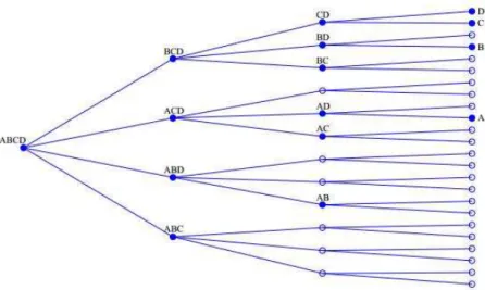
2.3.2 Autometrics’ Selection Algorithm
Figure 1: Tree for Possible Models.
The algorithm runs through the tree, following the nodes from left to right and from top to bottom, so that, in the above Figure example, it would pass through the models ABCD, BCD, CD, D, C, BD and so on. In each node, the variables are ordered in crescent order of significance, that is, in the GUM, A is the least significant variable and D is the most significant. It is possible that, in the following node, the order will be changed. For example, if C is less significant than B, the ordering would be given by CBD and the variable to be eliminated would be C.
If all the nodes from the tree were evaluated, the computational cost would be very large (for n regressors, 2n models would be estimated), so a number of strategies to jump the irrelevant nodes are used. These strategies are classified by Doornik(2009) as Pruning, Bunching, Chopping and Model Contrast.
Pruning consists in ignoring the nodes derived from a node invalidated by a diagnostic test or by backtesting (a joint significance F-test with relation to the initial GUM). If, e.g., starting from BCD, variable B cannot be eliminated, models CD, D and C are not estimated. The p-value used is denoted pa.
Bunching stems from the idea that it is possible, instead of eliminating the variables individually based in a t-test, eliminating groups of variables based in a F-test with relation to the current node. The size of the group is defined as default pb =max{12pa1/2, p3a/4}5. The F-tests significance level is the same as Pruning’s, i.e., pa. Once the group of variables is eliminated, we get to the correspondent following, avoiding estimation of many models. In the example of Figure 1, if we are at BCD and are able to effectively eliminate jointly B and C, the next model to be estimated is that containing only D, so that CD, C, BD, B and BC are ignored. If, in group, the variables cannot be withdrawn, we test the removal of groups with less variables, until a valid reduction is achieved.
Chopping means ignoring models, in a given ramification from a node, containing some variable or group of variables if they are of very little significance. For example, if we are, again, in BCD and BC presents a F-test with a greater p-value than a certainpc, the algorithm will estimate, in this ramification of the tree, only model D and will go next to node ACD.
5
The standad p-value used by Autometrics ispc =pb.
Model Contrasts consist in the elimination or shortening of paths in a certain ramification of the tree if it contains some terminal already found previously, so that it jumps to the nodes possessing possible terminals not yet estimated. As an example, suppose that, in the above Figure, we had selected D as a terminal in the first ramification. In the next step, ACD, the following node, AD, would originate two possible models: A and D. As D was already selected, the algorithm tests directly a reduction of ACD to A, speeding the calculations.
There are two types of Model Contrast: Union Contrast and Terminal Contrast. In the first, used when the current GUM is different from the previous GUM, the program considers, to jump, nodes that lead to any model different from the terminal union. In the second, used when the current GUM equals the previous, the jumped nodes takes into account paths that lead to terminals different from each one of the previously individually found terminals.
Several specification tests are then performed. However, differently from the algorithms cited earlier, in Autometrics they are performed only when the terminals are attained. If some test fail in some terminal, the program follows the path backwards from the node, making specification tests until some valid terminal is found. The tests performed are: residuals normality (Jarque and Bera, 1980), second order residual autocorrelation (χ2 test,
test, Godfrey (1978), Breusch & Pagan (1980)), autocorrelated conditional heteroscedasticity (ARCH) to second order (Engle, 1982) and that of in-sample stability (Chow, 1960).
In each iteration of the GUM, Autometrics divides the search in two stages. In the first, it ignores paths whose nodes contain terminals. In the second, it follows the root paths which contain terminals, using Model Contrast to reach definitive terminals more quickly.
Furthermore, before initializing the algorithm per se, there is the option of performing a pre-search to eliminate sets of lags. The default procedure is described as follows. First, group all variables with lagm, if none of the variables has p-value inferior tomax{p∗
p,1(kp), ps} - whereps =f(pa,0.2)≈5p0a.8,f(p, α) = αpif 0.94≤1 +p(α−1)≤1.06, f(p, α) =
αp
1+p(α−1),
otherwise; p∗
p,1(kp) = 1−(1−pp,1)kp, where kp is the number of regressors in question -, if the conjoint F-test’s p-value is superior topp and if the backtesting and diagnostic tests are respected, then exclude all the regressors and make the same with the lag m−1. Proceed with the sabe process until it is not possible to exclude variables.
Finally, when all the tree paths are covered, the final terminals where specification tests failed are discarded and, after the GUM convergence, the terminal with the minimum SIC is chosen.
In simulated experiments, models are evaluated based in the concepts of gauge, which measures the percentage of irrelevant variables retained in the model, of power, measuring the retention of relevant variables, and of the Root Mean Squared Error (RMSE) magnitude. The closer to 1 is the power, the closer to zero is the gauge and the smaller is the RMSE, the better the mechanism will be.
2.3.3 Modeling with more Variables than Observations
which could possibly affect the dependent variable.
Trying to estimate the GUM this way is obviously inviable, because there are more vari-ables than observations. Autometrics, however, utilizes a technique to reduct these models, initially proposed by Hendry & Krolzig (2005) and applied to the IIS context by Santos et al. (2008).
In case no variables beside the dummies are included, the first step is to apply the reduc-tion mechanism described above only with the T/2 first dummies, so that the resulting model will contain a subset of them. After this, the same is done with only the T/2 last dummies. Thus, we will obtain two models containing subsets of the initial dummies, the union of these models will generate a new GUM. Applying once more the reduction mechanism, we obtain the model containing the relevant dummies.
A generalization of this method can be applied when step dummies — which assume value 0 up to observation t−1 and 1 in the following observations — and other exogenous variables are included in the GUM. In this case, the algorithm introduced by Hendry & Johansen (2012) assumes N =PNj=1nj regressors so that N > T and nj < T for allj, that is, theN regressors are partitioned in portions smaller than the sample size.
Once the best fitted model is found, with relevant variables and dummies, the forecast is made in the standard way,i.e., the model’s n-steps ahead mathematical expectation.
2.4
Forecast Comparison (Diebold and Mariano Test)
To compare the forecasts, it will be used the Diebold & Mariano (1995) test, which utilizes the forecast errors from two different models to evaluate if on forecast is statistically superior the other.
For the test to be valid, it suffices that assumptions are made about the forecast errors and it is not necessary to make hypotheses about the models being tested, so that it is possible to compare even predictions that do not come from models.
The key hypothesis is made about the difference between the loss function associated with the forecast errors. Let eit be the forecast error from model i in period t, g(eit) some loss function, e.g. g(eit) = e2
it or g(eit) = |eit|, and dt = g(eit)−g(ejt) the loss function differential, it is assumed that dt is covariance-stationary:
E(dt) = µ,∀t
cov(dt, dt−τ) =ϕ(τ),∀t
V(dt) = σ2
d <∞
The hypothesis of equal predictive capacity is equivalent to E(dt) = 0. In this case, the test statistics is:
DM = d
ˆ
σd
d −
→N(0,1) (40)
whered= 1
T PT
t=1(g(eit)−g(ejt)) and ˆσd is a consistent estimator for the standard deviation of d.
q
2πfˆd(0)/T, where ˆfd(0) is a consistent estimator for the spectrum of the loss differential at frequency zero. fd(0) = 21πP∞τ=−∞ϕ(τ).
One caveat must be made concerning this method. Its objective is to test if different predictions from diverse sources are statistically different and, for this, it uses as primitive the forecast error loss function differential. When we compare two models, saving a fraction of the sample to calculate the loss function, what is used as primitives for the Diebold and Mariano test are, ultimately, the estimated parameters of the model, which origin the forecasts and, thus, the forecast errors. In doing so, part of the sample is lost, increasing the estimation uncertainty and jeopardizing efficiency in small samples.
Diebold (2012) argues that there are consolidated methods using the whole sample, as LR, LM and Wald tests, which are more efficient in model comparison. In the Bayesian context, the best model selection criterion resumes to that with the largest marginal likelihood function, that, as shown in Schwarz (1978), corresponds asymptotically to the model with smallest SIC. In fact, in the Gaussian linear regression context, Schwarz information criterion can be written as SIC = T(k/T)M SF E, where M SF E = PTt=1e2t
T , that is, the SIC is an estimate of the out-of-sample MSFE.
This work, however, is not intended to compare different models, but different methods of prediction. At each forecast step it is specified and estimated a new model, and thus there is not a unique SIC to be calculated and it is not possible to perform LR, LM or Wald tests. Therefore, Diebold and Mariano test arrive as the most appropriate test, since it uses only the series of loss differentials from each model.
3
Data and Period of Analysis
This work aims to evaluate the performance of nonlinear forecast techniques, mainly in periods where it is probable to exist structural breaks. So, the variable used here, which is very volatile and has asymmetric behavior, is the Brazilian monthly general industrial production quantum (mean 2002=100), measured by the Brazilian Institute of Geography and Statistics (IBGE) and the forecast horizon will start two periods before the subprime crisis reaches the series, that is, September 2008.
The series start in January 1975 and, in February 2014, it changes methodology. We will therefore use this period of analysis to avoid that structural breaks come from this change. The forecast horizon will be thus from September 2008 to February 2014, comprising a total of 66 periods, in which the forecasts will be real-time, that is, always one-step ahead, re-specifying and re-estimating at each step.
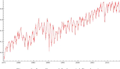
Figure 2 shows a graph with the complete series in natural logarithm. It is easily noticed the presence of non-stationarity and seasonality. To deal with these characteristics, the series is differenced with relation to the same month in the previous year, which would correct both problems. Figure 3 shows a graph with the treated series.
In STAR models,γ estimation becomes difficult if the probability of crossing the threshold
Since we used a twelve month difference to treat the data, we will supposeE[∆∆12xt] = 0 instead of E[∆2xt] = 0 in the double differencing device and denote it DD12, i.e. the
industrial production growth in respect to the same month of the previous year do not continuously accelerate. This modification is straightforward and the interpretation is not impaired.
Figure 2: Log General Industrial Production
Figure 3: Log General Industrial Production - Annual Difference
4
Results
The following results show the original series (D12Lgeneralind) and one-step ahead forecasts graphs, in which is shown only the prediction horizon.
d is estimated using linearity tests and the nonlinear model parameters are estimated by nonlinear least squares.
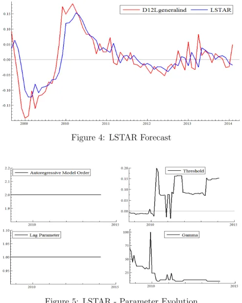
Figure 4: LSTAR Forecast
Figure 5: LSTAR - Parameter Evolution
In Figure 5, which shows the LSTAR parameters evolution, we see that the autoregressive order and the lag parameter remain constant through all the forecast horizon. The gamma parameter, the speed of transition, decreases over time. The threshold starts near the intuitive value of zero in the first year and a half, when there is a drop in the industrial production. After this, however, when the series abnormally increases and subsequently returns to a more stable behavior, the threshold becomes erratic and then stays at high levels, so that from March 2011 on, the series does not cross it, that is, it stays in the lower regime for the remain of the forecast horizon.
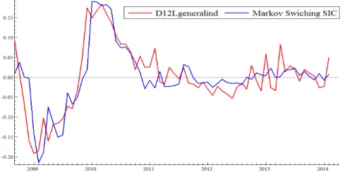
switching variance and are described as follows. Models with 2 regimes, one to twelve fixed lags; with 2 regimes, one to twelve lags varying with regimes. Models with 3 regimes, one to twelve fixed lags; and 3 regimes, one to twelve varying lags. Besides these, models with only the intercept were estimated for 2 and 3 regimes. The results are shown in Figure 6.
Figure 6: MSAR SIC Forecast
The forecasts seem to be more volatile than the actual series and goes in an opposite direction in some periods after the end of 2010.
Figure 7 shows the results of the model with dummy saturation. As variables in the GUM, 12 lags (which is the maximum number of lags considered for selection for the AR(p) model with the Schwarz Criterion) of the dependent variable are added, as well as the impulse and step dummies for each observation.
Figure 7: Dummy Saturation Forecast - Indicator and Step Dummies
new observation in each new forecast, it is not possible to know if the discrepant value is from an outlier or from a level shift.
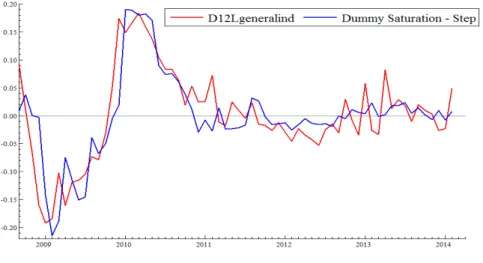
To investigate this possibility, a model only with step dummy saturation and lags was estimated, so that the Autometrics selection mechanism will interpret a discrepant observa-tion necessarily as a level shift, corroborating or refuting this possibility according with the following observations. Figure 8 displays this formulation’s forecasts:
Figure 8: Dummy Saturation Forecast - Step Dummies Only
The forecasts are able get closer to the original series in the initial periods in which it decreases and, after that, it abruptly grows, and have similar precision in posterior periods. This result corroborate with the expected and can suggest that, in case there is a kind of dummy saturation which interprets new discrepant observations as level shifts at the same time it models past outliers with impulse dummies, we will get better predictions.
Next, in Figures 10 and 9, respectively, are the forecasts from naive models, namely, the Double Difference Device (DD12), and the autoregressive model of order p (AR(p)), which defines at each forecast step a new lag order, wherepis selected at each observation with the Schwarz Criterion.
Figure 10: Double Difference Forecast
AR(p) seems to follow the true series similarly to the LSTAR model, although not reacting as much as it should in period of crisis. The DD12, on the other hand, only repeats the previous D12Lgeneralind variation value.
The table below shows a summary of results containing the Medium Forecast Error (MFE), the RMSFE and the MAPFE for each method.
Mtodo RMSFE MAPFE MFE
LSTAR 0.04673 100.033% 0.00371 MSAR-BIC 0.04753 109.010% 0.00318 DSAT 0.04950 104.760% 0.00488 DSAT-step 0.04563 89.327% -0.00071 AR(p) 0.04468 93.937% 0.00008 DD12 0.04548 118.961% -0.00045
Table 1: Result Summary
Considering the MFE, none of the predictors have a large bias, where AR(p) has the smal-lest, followed closely by DD12 and DSAT-step. With respect to RMSFE, AR(p) dominate the others, although the results of DSAT-step and DD12 are close to AR(p)’s. Concerning the MAPFE, on the other hand, DSAT-step dominates the others, followed by AR(p).
It is worth noting that, with respect to the Dummy Saturation model, the fact that the DSAT’s RMSFE and MAPFE are larger than DSAT-step’s must arrive from the fact that we cannot distinguish, in the last periods, if the discrepant observations come from a impulse or a step dummy, i.e., from an outlier or a level shift. In the DSAT-step case, RMSFE and MAPFE decrease, which is evidence in favor of this hypothesis.
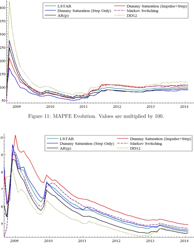
Figure 11: MAPFE Evolution. Values are multiplied by 100.
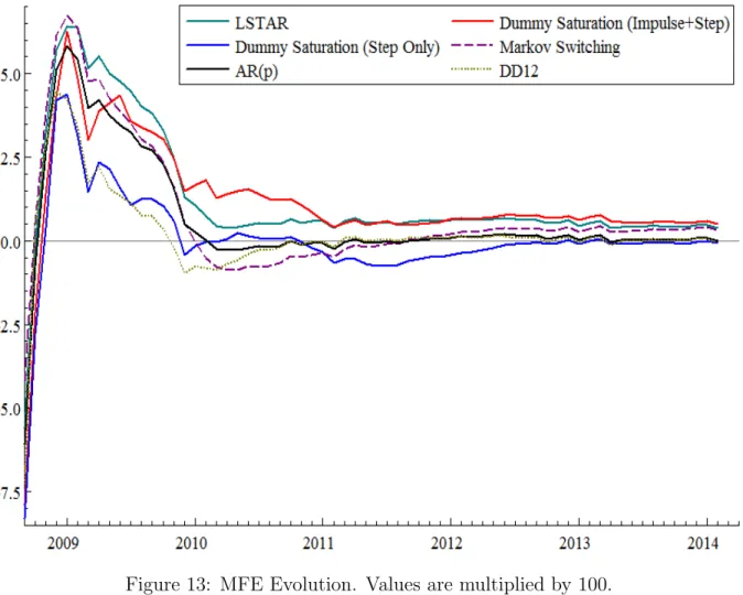
Figure 13: MFE Evolution. Values are multiplied by 100.
We see in Figure 11 that, for all the models, the MAPFE is high in the first periods, because of the low number of observations to calculate this statistic and the possible structural break in the series in the initial periods of the forecast horizon. In the following months, all MAPFE’s keep decreasing until 2011, when it increases, converging to the final values presented in Table 1 as the series becomes more stable.
Looking at Figure 12, it is shown that, probably for the same motives as the MAPFE, the RMSFE is high and decreases in the first periods. After the soaring of the growth in industrial production after 2010, all RMSFE’s suffer a shift up and then decreases, converging to its final values in February 2014. DD12 forecasts dominates the rest of the models until the last year of the forecast horizon, which is evidence that this naive performs better in turbulent periods (those in which there are possible structural breaks).
In contrast, DD12 MAPFE is higher than the rest. This happens because the RMSFE punishes high deviations more severely, while the MAPFE does not. Therefore, we can conclude that DD12 misses frequently the target, but seldom at great magnitudes, at least up to the last year of the forecast horizon.
sample. In contrast with DD12, DSAT-step predicts frequently near the actual series, but, when it does not, it misses badly.
Figure 13 shows the MFE evolution (predicted value minus realized value). All methods presents a positive bias after the first period, which reflects the industrial production verti-ginous plunge between November 2008 and November 2009. In 2010, when the production begins to grow more than the unconditional mean, the bias tends to be corrected. Some methods, as Markov Switching and DD12, present a negative bias in the periods of high growth in 2010, returning to near zero bias after the following year.
To verify if forecasts are statistically different, we perform the Diebold and Mariano test for all the forecast horizons starting in September 2008, in the same way that in Figures 11, 12 and 13. We made the test for all model against the two naive models — DD12 and AR(p) — for two loss functions: MAPFE and MSFE. However, we display here only those results in which the test returns values that reach p-values smaller than the standard significance level of 5%, displaying the rest in the appendix. The results are exhibited in Figures 14, 15 and 16.
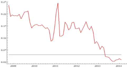
Figure 15: Diebold-Mariano p-value: Alternative Hypothesis - DSAT-step ¿ DD12, Loss Function: MAPFE. Horizontal line is the significance level of 5%.
Figure 16: Diebold-Mariano p-value: Alternative Hypothesis - LSTAR ¿ DD12, Loss Func-tion: MAPFE. Horizontal line is the significance level of 5%.
With MAPFE as loss function, forecasts of LSTAR and of DSAT-step are superior, with the standard significance level of 5% (horizontal line), to the naive method DD12 for the forecast horizons ending from the beginning of 2013 to the end of the sample. Moreover, forecasts of AR(p) are superior to those of DD12 in a larger set of forecast horizons.
However, no nonlinear model has superior predictive accuracy over the AR(p) forecasts and neither over the DD12 forecasts if we use the MSFE as loss function.
5
Conclusion
probably structural breaks. The models analyzed are the Markov Switching Autoregress-ive, the Logistic Smooth Transition Autoregressive and the automatic selection algorithm Autometrics with Dummy Saturation.
The series used here was the Brazilian monthly general industrial production quantum, annually differenced to avoid problems of non-stationarity and seasonality. The sample begins in January 1975 and ends in February 2014. The forecast horizon starts two periods before the subprime crisis reaches the series, in September 2008.
The estimation was done one-step ahead and real-time, that is, with each new observation in the forecast horizon, a new specification was made, the model was re-estimated and a prediction was made for the following month.
The results show that AR(p) has the smallest root mean squared forecast error and the dummy saturation with only step dummies has the smallest mean absolute percentage forecast errors. To test if these outcomes were caused by chance and if it was different in the more turbulent years of the sample (the first two and a half years), Diebold & Mariano (1995) test was performed for all possible forecast horizons beginning in September 2008.
6
References
Arango, L. & Gonzalez, A. (2001). Some evidence of smooth transition nonlinearity in Colombian inflation. Applied Economics, 33(2):155-162.
Bardsen, G., Hurn, S., & McHugh, Z. (2012). Asymmetric unemployment rate dynamics in Australia. Studies in Nonlinear Dynamics & Econometrics, 16(1):1-22.
Bontemps, C. & Mizon, G. E. (2003). Congruence and encompassing. In Stigum, B., editor,Econometrics and the Philosophy of Economics, pages 354-378. Princeton University Press, New Jersey.
Breusch, T. S. & Pagan, A. R. (1980). The Lagrange multiplier test and its applications to model specification in econometrics. The Review of Economic Studies, 47(1):239-253.
Castle, J. L., Doornik, J. A., & Hendry, D. F. (2012). Model selection when there are multiple breaks. Journal of Econometrics, 169(2):239-246.
Castle, J. L., Fawcett, N. W., & Hendry, D. F. (2010). Forecasting with equilibrium-correction models during structural breaks. Journal of Econometrics, 158(1):25-36.
Castle, J. L., Fawcett, N. W., & Hendry, D. F. (2011). Forecasting breaks and forecasting during breaks. Discussion Paper 535, University of Oxford, Oxford.
Castle, J. L. & Hendry, D. F. (2013). Semi-automatic non-linear model selection. Dis-cussion Paper 654, University of Oxford, Oxford.
Chow, G. C. (1960). Tests of equality between sets of coefficients in two linear regressions.
Econometrica, 28(3):591-605.
Clements, M. & Hendry, D. (1998). Forecasting economic time series. Cambridge Uni-versity Press, Cambridge.
Clements, M. P. & Hendry, D. F. (2008). Economic forecasting in a changing world.
Capitalism and Society, 3(2). Article 1.
Davies, R. B. (1977). Hypothesis testing when a nuisance parameter is present only under the alternative. Biometrika, 64(2):247-254.
Deschamps, P. J. (2008). Comparing Smooth Transition and Markov Switching autore-gressive models of US unemployment. Journal of Applied Econometrics, 23(4):435-462.
Diebold, F. X. (2012). Comparing predictive accuracy, twenty years later: A personal perspective on the use and abuse of Diebold-Mariano tests. Journal of Business & Economic Statistics, 33(1):1-24.
Diebold, F. X. & Mariano, R. S. (1995). Comparing predictive accuracy. Journal of
Business & Economic Statistics, 13(3):253-263.
Doornik, J. A. (2009). Autometrics. In Castle, J. L. and Shephard, N., editors, The
Methodology and Practice of Econometrics, pages 88-121. Oxford University Press, Oxford.
Engel, C. (1994). Can the Markov Switching Model forecast exchange rates? Journal of
International Economics, 36(1):151-165.
Engle, R. F. (1982). Autoregressive conditional heteroscedasticity with estimates of the variance of United Kingdom inflation. Econometrica, 50(4):987-1007.
Godfrey, L. G. (1978). Testing for higher order serial correlation in regression equations when the regressors include lagged dependent variables. Econometrica, 46(6):1303-1310.
Hamilton, J. D. (1990). Analysis of time series subject to changes in regime. Journal of
Econometrics, 45(1):39-70.
Hamilton, J. D. (1994). Time Series Analysis. Princeton University Press, New Jersey. Hendry, D. F. (1995). Dynamic econometrics. Oxford University Press, Oxford.
Hendry, D. F. (2000). On detectable and non-detectable structural change. Structural
change and economic dynamics, 11(1):45-65.
Hendry, D. F. (2006). Robustifying forecasts from equilibrium-correction systems. Journal
of Econometrics, 135(1):399-426.
Hendry, D. F. (2012). Mathematical models and economic forecasting: Some uses and misuses of mathematics in economics. In Dieks, D., Gonzalez, W. J., Hartmann, S., Stltzner, M., and Weber, M., editors, Probabilities, Laws, and Structures, pages 319-335. Springer.
Hendry, D. F. & Johansen, S. (2012). Model discovery and Trygve Haavelmo’s legacy. Discussion Paper 598, University of Oxford, Oxford.
Hendry, D. F. & Krolzig, H.-M. (1999). Improving on ‘Data mining reconsidered’by K.D. Hoover and S.J. Perez. The Econometrics Journal, 2(2):202-219.
Hendry, D. F. & Krolzig, H.-M. (2005). The properties of automatic GETS modelling.
The Economic Journal, 115(502):C32-C61.
Hendry, D. F. & Mizon, G. E. (2011). Econometric modelling of time series with outlying observations. Journal of Time Series Econometrics, 3(1). Article 1.
Hoover, K. D. & Perez, S. J. (1999). Data mining reconsidered: encompassing and the general-to-specific approach to specification search. The Econometrics Journal, 2(2):167-191. Jarque, C. M. & Bera, A. K. (1980). Efficient tests for normality, homoscedasticity and serial independence of regression residuals. Economics letters, 6(3):255-259.
Kim, C.-J. (1994). Dynamic linear models with Markov-switching. Journal of Economet-rics, 60(1):1-22.
Lovell, M. C. (1983). Data mining. The Review of Economics and Statistics, 65(1):1-12. Lundbergh, S. & Ter¨asvirta, T. (2005). Forecasting with Smooth Transition Autoregress-ive models. In Clements, M. P. and Hendry, D. F., editors, A Companion to Economic
Forecasting, pages 485-509. Wiley-Blackwell, New Jersey.
Luukkonen, R., Saikkonen, P., & Ter¨asvirta, T. (1988). Testing linearity against smooth transition autoregressive models. Biometrika, 75(3):491-499.
Mizon, G. E. (1995). Progressive modeling of macroeconomic time series: The LSE methodology. In Advanced Lectures in Quantitative Economics, volume 2, pages 184-205. Academic Press, New York.
Montgomery, A. L., Zarnowitz, V., Tsay, R. S., & Tiao, G. C. (1998). Forecasting the US unemployment rate. Journal of the American Statistical Association, 93(442):478-493.
¨
Ocal, N. & Osborn, D. R. (2000). Business cycle non-linearities in UK consumption and production. Journal of Applied Econometrics, 15(1):27-43.
Santos, C., Hendry, D. F., & Johansen, S. (2008). Automatic selection of indicators in a fully saturated regression. Computational Statistics, 23(2):317-335.
Schwarz, G. (1978). Estimating the dimension of a model. The Annals of Statistics, 6(2):461-464.
Ter¨asvirta, T. (1994). Specification, estimation, and evaluation of Smooth Transition Autoregressive Models. Journal of the American Statistical Association, 89(425):208-218.
Ter¨asvirta, T. & Anderson, H. M. (1992). Characterizing nonlinearities in business cycles using smooth transition autoregressive models. Journal of Applied Econometrics, 7:S119-S136.
Wooldridge, J. M. (1994). Estimation and inference for dependent processes. In Engle, R. F. and McFadden, D. L., editors, Handbook of Econometrics, volume 4, pages 2639-2738. Elsevier.
Appendix
Diebold and Mariano Tests Results
The Figures below show the p-value evolution of the Diebold and Mariano test in all forecast horizons which start in September 2009 (that is, the first is 2008.9-2008.10 and the last is 2008.9-2014.2). All methods analyzed are tested against the two naive methods AR(p) and DD12. No null hypothesis is rejected, except for AR(p), DSAT-step and LSTAR against DD12, all using the MAPFE loss function.
Figure A.1: Diebold-Mariano p-value: Alternative Hypothesis - DD12 ¿ AR(p), Loss Func-tion: MAPFE. Horizontal line is the significance level of 5%.
Figure A.3: Diebold-Mariano p-value: Alternative Hypothesis - DSAT-step ¿ AR(p), Loss Function: MAPFE. Horizontal line is the significance level of 5%.
Figure A.4: Diebold-Mariano p-value: Alternative Hypothesis - LSTAR ¿ AR(p), Loss Func-tion: MAPFE. Horizontal line is the significance level of 5%.
Figure A.6: Diebold-Mariano p-value: Alternative Hypothesis - DD12 ¿ AR(p), Loss Func-tion: RMSFE. Horizontal line is the significance level of 5%.
Figure A.7: Diebold-Mariano p-value: Alternative Hypothesis - DSAT ¿ AR(p), Loss Func-tion: RMSFE. Horizontal line is the significance level of 5%.
Figure A.9: Diebold-Mariano p-value: Alternative Hypothesis - LSTAR ¿ AR(p), Loss Func-tion: RMSFE. Horizontal line is the significance level of 5%.
Figure A.10: Diebold-Mariano p-value: Alternative Hypothesis - Markov ¿ AR(p), Loss Function: RMSFE. Horizontal line is the significance level of 5%.
Figure A.12: Diebold-Mariano p-value: Alternative Hypothesis - DSAT ¿ DD12, Loss Func-tion: MAPFE. Horizontal line is the significance level of 5%.
Figure A.13: Diebold-Mariano p-value: Alternative Hypothesis - DSAT-step ¿ DD12, Loss Function: MAPFE. Horizontal line is the significance level of 5%.
Figure A.15: Diebold-Mariano p-value: Alternative Hypothesis - Markov ¿ DD12, Loss Func-tion: MAPFE. Horizontal line is the significance level of 5%.
Figure A.16: Diebold-Mariano p-value: Alternative Hypothesis - AR(p) ¿ DD12, Loss Func-tion: RMSFE. Horizontal line is the significance level of 5%.
Figure A.18: Diebold-Mariano p-value: Alternative Hypothesis - DSAT-step ¿ DD12, Loss Function: RMSFE. Horizontal line is the significance level of 5%.
Figure A.19: Diebold-Mariano p-value: Alternative Hypothesis - LSTAR ¿ DD12, Loss Func-tion: RMSFE. Horizontal line is the significance level of 5%.