Anomaly mediated supersymmetry breaking without R-parity

Anomaly mediated supersymmetry breaking

without

R

-parity

F. de Campos

_{, M.A. Díaz}

_{, O.J.P. Éboli}

_{, M.B. Magro}

_,

P.G. Mercadante

a_{Departamento de Física e Química, Universidade Estadual Paulista, Av. Dr. Ariberto Pereira da Cunha 333,}

Guaratinguetá, SP, Brazil

b_{Departamento de Física, Universidad Católica de Chile, Av. Vicuña Mackenna 4860, Santiago, Chile} c_{Instituto de Física, Universidade de São Paulo, CP 66.318, 05389-970, São Paulo, SP, Brazil}

Received 9 October 2001; accepted 4 December 2001

Abstract

We analyze the low energy features of a supersymmetric standard model where the anomaly-induced contributions to the soft parameters are dominant in a scenario with bilinear R-parity violation. This class of models leads to mixings between the standard model particles and supersymmetric ones which change the low energy phenomenology and searches for supersymmetry. In addition,R-parity violation interactions give rise to small neutrino masses which we show to be consistent with the present observations.2002 Elsevier Science B.V. All rights reserved.

PACS: 12.60.Jv; 14.60.Pq; 14.80.Ly

1. Introduction

Supersymmetry (SUSY) is a promising candidate for physics beyond the Standard Model (SM) and there is a large ongoing search for supersymmetric partners of the SM particles. However, no positive signal has been observed so far. Therefore, if supersymmetry is a symmetry of nature, it is an experimental fact that it must be broken. The two best known classes of models for supersymmetry breaking are gravity-mediated [1] and gauge-gravity-mediated [2] SUSY breaking. In gravity-gravity-mediated models, SUSY is assumed to be broken in a hidden sector by fields which interact with the visible particles only via gravitational interactions and not via gauge or Yukawa interactions. In

gauge-E-mail address: [email protected] (M.B. Magro).

mediated models, on the contrary, SUSY is broken in a hidden sector and transmitted to the visible sector via SM gauge interactions of messenger particles.

There is a third scenario, called anomaly-mediated SUSY breaking [3], which is based on the observation that the super-Weyl anomaly gives rise to loop contribution to sparticle masses. The anomaly contributions are always present and in some cases they can dominate; this is the anomaly mediated supersymmetry breaking (AMSB) scenario. In this way, the gaugino masses are proportional to their corresponding gauge group

β-functions with the lightest SUSY particle being mainly wino. Analogously, the scalar masses and trilinear couplings are functions of gauge and Yukawaβ-functions. Without further contributions the slepton squared masses turn out to be negative. This tachyonic spectrum is usually cured by adding an universal non-anomaly mediated contribution

m2₀>0 to every scalar mass [4].

So far, most of the work on AMSB has been done assuming R-parity (RP)

conservation [5–7]; see [8] for an exception.R-parity violation [9] has received quite some attention lately motivated by the Super-Kamiokande Collaboration results on neutrino oscillations [10], which indicate neutrinos have mass [11]. One way of introducing mass to the neutrinos is via bilinear R-parity violation (BRpV) [12], which is a simple and predictive model for the neutrino masses and mixing angles [13,14]. In this work, we study the phenomenology of an anomaly mediated SUSY breaking model which includes bilinear R-parity violation (AMSB-BRpV), stressing its differences to the R-parity conserving case.

In BRpV-MSSM [15], bilinear R-parity and lepton number violating terms are introduced explicitly in the superpotential. These terms induce vacuum expectation values (vev’s)vi for the sneutrinos, and neutrino masses through mixing with neutralinos. At tree

level, only one neutrino acquires a mass [16], which is proportional to the sneutrino vev in a basis where the bilinearR-parity violating terms are removed from the superpotential. At one-loop, three neutrinos get a non-zero mass, producing a hierarchical neutrino mass spectrum [17]. It has been shown that the atmospheric mass scale, given by the heaviest neutrino mass, is determined by tree level physics and that the solar mass scale, given by the second heaviest neutrino mass, is determined by one-loop corrections [14].

In our model, the presence ofRP violating interactions gives rise to neutrino masses

which we show to be consistent with the present observations. Moreover, the low-energy phenomenology is quite distinct of the conservingR-parity AMSB scenario. For instance, the lightest supersymmetric particle (LSP) is unstable, which allows regions of the parameter space where the stau or the tau-sneutrino is the LSP. In our scenario, decays can proceed via the mixing between the standard model particles and supersymmetric ones. As an example, the mixing between the lightest neutralinoχ_˜10(charginoχ_˜1±) andντ (τ±)

allows the following decays

˜

χ₁0_→ντZ∗,

˜

χ₁0_→τ±W∓ ∗,

˜

χ₁±_→τ±Z∗,

˜

Another effect of the mixing between the standard model and supersymmetric particles is a sizeable change in the mass of the supersymmetric particles. For instance, the mixing between scalar taus and the charged Higgs can lead to an increase in the splitting between the two scalar tau mass eigenstates by a factor that can be as large as 10 with respect to the

RP conserving case.

This paper is organized as follows. We define in Section 2 our anomaly mediated SUSY breaking model which includes bilinearR-parity violation, stating explicitly our working hypotheses. This section also contains an overall view of the supersymmetric spectrum in our model. We study the properties of the CP-odd, CP-even, and charged scalar particles in Sections 3, 4, and 5, respectively, concentrating on the mixing angles that arise from the introduction of theR-parity violating terms. Section 6 contains the analysis that shows that our model can generate neutrino masses in agreement with the present knowledge. In Section 7 we provide a discussion of the general phenomenological aspects of our model while in Section 8 we draw our conclusions.

2. The AMSB-BRpV model

Our model, besides the usual RP conserving Yukawa terms in the superpotential,

includes the following bilinear terms

(1)

Wbilinear= −εab

µH_daH_ub₊ǫiLˆaiHub

,

where the second one violatesRP and we take|ǫi| ≪ |µ|. Analogously, the relevant soft

bilinear terms are

Vsoft=m2HuH

a∗

u Hua+m2HdH

a∗

d Hda+ML2iL˜

a∗

i L˜ai

(2)

−εab

BµH_daH_ub₊BiǫiL˜aiHub

,

where the terms proportional toBi are the ones that violatesRP. The explicitRP violating

terms induce vacuum expectation valuesvi,i=1,2,3 for the sneutrinos, in addition to the

two Higgs doublets vev’svuandvd. In phenomenological studies where the details of the

neutrino sector are not relevant, it has been proven very useful to work in the approximation whereRP and lepton number are violated in only one generation [18]. In these cases, a

determination of the mass scale of the atmospheric neutrino anomaly within a factor of two is usually enough, and that can be achieved in the approximation whereRP is violated

only in the third generation.

In this work we assume thatRP violation takes place only in the third generation, and

consequently the parameter space of our model is

(3)

m0, m3/2,tanβ,sign(µ), ǫ3, andmντ,

In AMSB models, the soft terms are fixed in a non-universal way at the unification scale which we assumed to beMGUT=2.4×1016 GeV; see Appendix A for details. We considered the running of the masses and couplings to the electroweak scale, assumed to be the top mass, using the one-loop renormalization group equations (RGE) that are presented in Appendix B. In the evaluation of the gaugino masses, we included the next-to-leading order (NLO) corrections coming fromαs, the two-loop top Yukawa contributions to the

beta-functions, and threshold corrections enhanced by large logarithms; for details see [4]. The NLO corrections are especially important forM2, leading to a change in the wino mass by more than 20%.

One of the virtues of AMSB models is that the SU(2)_⊗U (1) symmetry is broken radiatively by the running of the RGE from the GUT scale to the weak one. This feature is preserved by our model since the one-loop RGE are not affected by the bilinearRP

violating interactions; see Appendix B. In our model, the electroweak symmetry is broken by the vacuum expectation values of the two Higgs doubletsHd andHu, and the neutral

component of the third left slepton doubletL˜3. We denote these fields as

Hd=

_√1 2

χ_d0₊vd+iϕd0

H_d−

, Hu=

_H+ u 1 √ 2 χ0

u+vu+iϕu0

,

(4)

˜

L3=

_√1 2

˜

ν_τR₊v3+iν˜τi0

˜

τ−

.

The above vev’svi can be obtained through the minimization conditions, or tadpole

equations, which in the AMSB-BRpV model are

t_d0₌m2_H

d+µ 2_v

d−Bµvu−µǫ3v3+ 1 8

g2₊g′2vd

v_d2₋v_u2₊v2₃, t_u0₌m2_Hu+µ2₊ǫ₃2vu−Bµvd+B3ǫ3v3−

1 8

g2₊g′2vu

v_d2₋v_u2₊v2₃,

(5)

t₃0₌m2_L

3+ǫ 2 3

v3−µǫ3vd+B3ǫ3vu+

1 8

g2₊g′2v3v2_d−v2u+v32

,

at tree level. At the minimum we must imposet_d0₌t_u0₌t₃0₌0. In practice, the input parameters are the soft massesmHd, mHu, andmL3, the vev’svu,vd, andv3 (obtained frommZ, tanβ, andmντ), andǫ3. We then use the tadpole equations to determineB,B3, and_|µ_|.

One-loop corrections to the tadpole equations change the value of _|µ_| by O(20%), therefore, we also included the one-loop corrections due to third generation of quarks and squarks [17]:

(6)

ti=ti0+Ti(Q),

whereti, withi=d, u, are the renormalized tadpoles,t_i0are given in (5), andTi(Q)are

the renormalized one-loop contributions at the scaleQ. Here we neglected the one-loop corrections fort3since we are only interested in the value ofµ.

Fig. 1. Supersymmetric mass spectrum in AMSB-BRpV form3/2=32 TeV, tanβ=5, andµ <0. The values of

ǫ3andmντ were randomly varied according to 10−5< ǫ3<1 GeV and 10−6< mντ<1 eV.

m3/2=32 TeV, tanβ=5, andµ <0, varyingǫ3andmντaccording to 10− 5_{< ǫ}

3<1 GeV and 10−6< mντ <1 eV. The widths of the scatter plots show that the spectrum exhibits a very small dependence onǫ3andmντ. Throughout this paper we use this range forǫ3and

mντ in all figures.

We can see from this figure that, form0200 GeV, the LSP is the lightest neutralino

˜

χ₁0 with the lightest chargino χ_˜1+ almost degenerated with it, as in RP-conserving

AMSB. Nevertheless, the LSP is the lightest stau τ_˜1+ for m0 200 GeV. This last region of parameter space is forbidden inRP-conserving AMSB, but perfectly possible in

AMSB-BRpV since the stau is unstable, decaying intoRP-violating modes with sizeable

branching ratios. Furthermore, the slepton masses have a strong dependence onm0. We plotted masses of the two staus, which have an appreciable splitting, the almost degenerated smuons, and the closely degenerated tau-sneutrinos.1The heavy Higgs bosons have also a strong dependence onm0and, for the chosen parameters, they are much heavier than the sleptons. On the other hand, the gauginos show little dependence onm0, as expected.

Bounds on BRpV parameters depend in general on supersymmetric masses and couplings, as shown in [19]. In models with BRpV in only one generation it is possible to estimate the bound onǫ3in a much simpler way: if we rotate the lepton and Higgs fields such that the bilinear term in the superpotential is eliminated [20], a trilinear termλ′ is generated

(7)

λ′_3ii=hdi

ǫ3

µ2_+ǫ2 3

,

wherehdiis the Yukawa coupling of the down quark of theith generation. Bounds on these couplings can be found on [9]:

(8)

λ′₃₁₁<0.11_× md˜R

100 GeV, λ ′

322<0.52×

m_˜sR

100 GeV, λ ′

333<0.45,

and, considering the values of the Yukawa couplings, it is easy to see that these bounds are satisfied for our choiceǫ3<1 GeV.

3. CP-odd Higgs/sneutrino sector

In our model, the CP-odd Higgs sector mixes with the imaginary part of the tau-sneutrino due to the bilinearRP violating interactions. Writing the mass terms in the form

(9)

Vquadratic= 1 2

ϕ_d0, ϕ_u0,ν_˜τi0M2

P0  

ϕ_d0 ϕ_u0

˜

νi_τ0  , we have M2 P0 =    

m2_A(0)s_β2₊µǫ3v_v3

d m

2(0)

A sβcβ −µǫ3

m_A2(0)sβcβ mA2(0)c2β−µǫ3_vv3_d

c2 β

s2 β +

v₃2 v2 d c2 β s2 β ¯

m2_ν˜

τ −µǫ3

cβ

sβ +

v3

vd

cβ

sβm¯ 2 ˜

ντ

−µǫ3 −µǫ3

cβ

sβ +

v3

vd

cβ

sβm¯ 2 ˜

ντ m¯

2 ˜ ντ    , (10)

withm_¯2_ν˜

τ =m 2(0)

˜

ντ +ǫ 2 3+ 1 8g 2 Zv 2 3andg

2

Z≡g

2

+g′2. Here,

(11)

m2_A(0)₌ Bµ sβcβ

and m2_ν˜(0)

τ =M 2

L3+ 1 8g

2

Z

v_d2₋v_u2

are, respectively, the CP-odd Higgs and sneutrino masses in the RP conserving limit

(ǫ3=v3=0). In order to write this mass matrix we have eliminatedm2_Hu,m2_H

This matrix can be diagonalized with a rotation

(12)

_A0

G0

˜

ν_τodd

=R_P0  

ϕ_d0 ϕ_u0

˜

ν_τi0  ,

whereG0is the massless neutral Goldstone boson. Between the other two eigenstates, the one with largestν_˜τi0component is called CP-odd tau-sneutrinoν_˜τoddand the remaining state is called CP-odd HiggsA0.

As an intermediate step, it is convenient to make explicit the masslessness of the Goldstone boson with the rotation

(13)

R

P0=  

sβ cβ 0

−cβr sβr −v_v3_dcβr

−v3

vdc 2

βr v3

vdsβcβr r

 ,

where

(14)

r₌ 1

1₊v 2 3

v2_dc

2

β

,

obtaining a rotated mass matrixR_P0M2

P0R T

P0 which has a column and a row of zeros, corresponding toG0. This procedure simplifies the analysis since the remaining 2_×2 mass matrix for(A0,ν_˜τodd)is

(15)

M2_P0=

  

m2_A(0)₊v

2 3 v2 d c4 β s2 β ¯

m2_ν˜

τ+µǫ3

v3

vd

s2 β−c2β

s2 β v3 vd c2 β

sβm¯ 2 ˜

ντ−µǫ3 1 sβ r v3 vd

c2_β sβm¯

2 ˜

ντ−µǫ3 1

sβ

r m_¯2_ν˜

τ 1 r2   .

We quantify the mixing between the tau-sneutrino and the neutral Higgs bosons through

(16) sin2θodd=

ν_˜τoddϕ_u02₊ν_˜τoddϕ_d02.

If we consider theRP violating interactions as a perturbation, we can show that

(17) sin2θodd≃

v3

vdc 2

βm

2(0)

˜

ντ −µǫ3

2

s2_βm_A2(0)₋m2_ν˜(0)

τ

2 +

v2 3

v2_dc

2

β,

indicating that this mixing can be large when the CP-odd Higgs bosonA0and the sneutrino

˜

ντ are approximately degenerate.

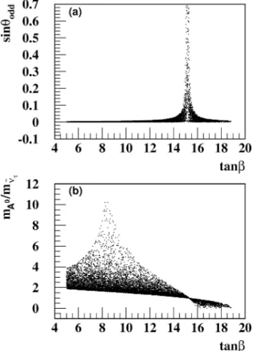
Fig. 2(a) displays the full sneutrino-Higgs mixing (16), with no approximations, as a function of tanβ form3/2=32 TeV,µ <0 and 100< m0<300 GeV. In a large fraction of the parameter space this mixing is small, since it is proportional to the BRpV parameters squared divided by MSSM mass parameters squared. However, it is possible to find a region where the mixing is sizable, e.g., for our choice of parameters this happens at tanβ_≈15. As expected, the region of large mixing is associated to near degenerate states, as we can see from Fig. 2(b) where we present the ratio between the CP-odd Higgs mass

mAand the CP-odd tau-sneutrino massmν_˜odd

Fig. 2. (a) CP-odd Higgs–sneutrino mixing and (b) ratio between the CP-odd Higgs mass and the sneutrino mass as a function of tanβform3/2=32 TeV,µ <0 and 100< m0<300 GeV.

4. CP-even Higgs/sneutrino sector

The mass terms of the CP-even neutral scalar sector are

(18)

Vquadratic= 1 2

χ_d0, χ_u0,ν_˜τr0M2

S0  

χ_d0 χ_u0

˜

ν_τr0  ,

where the mass matrix can be separated into two pieces

(19)

M2

S0=M 2(0) S0 +M

2(1) S0 .

The first term due toRP conserving interactions is

(20)

M2(0)

S0 =   

m_A2(0)s_β2₊1₄g_Z2v2_{d −}m_A2(0)sβcβ−₄1g2_Zvdvu 0

−m2_A(0)sβcβ−1₄gZ2vdvu m2A(0)c2β+14g 2

Zv2u 0

0 0 m2_ν˜(0)

τ

while the one associated to theRP violating terms is

M2(1)

S0

=

   

µǫ₃v3

vd 0 −µǫ3+

1 4g2Zvdv3

0 v

2 3

v2 d

c2 β

s2 β

m2_ν˜(0)

τ −µǫ3

v3

vd

c2 β

s2 β

µǫ3

cβ

sβ −

v3

vd

cβ

sβm 2(0)

˜

ντ − 1 4g

2

Zvuv3

−µǫ₃₊1₄g_Z2v_dv₃ µǫ₃c_sβ

β −

v3

vd

cβ

sβm 2(0)

˜

ντ − 1

4gZ2vuv3 ǫ32+ 3 8g2Zv32

   

(21)

Fig. 3. (a) CP-even Higgs–sneutrino mixing; (b) ratio between heavy CP-even Higgs and tau-sneutrino masses and (c) ratio between light CP-even Higgs and tau-sneutrino masses as a function of tanβform3/2=32 TeV,

Radiative corrections can change significantly the lightest Higgs mass and, consequently, we have also introduced the leading correction to its mass

(22)

/m_χ0 u≡

3m4_t

2π2_v2

uv′

ln

_m

˜

t1mt˜2

m2_t

,

with

(23)

v′₌1₋ v

2 3

v2_d+v2

u+v23

,

by adding it to the element_[M2

S0]22.

Analogously to the CP-odd sector, we define the mixing between the CP-even tau-sneutrino and the neutral Higgs bosons as

(24) sin2θeven=

ν_˜τevenχ_d02₊ν_˜τevenχ_u02₌H0ν_˜τr02₊h0ν_˜τr02.

In general, this mixing is small since it is proportional to the RP breaking parameters

squared, however, it can be large provided the sneutrino is degenerate either withh0orH0. In Fig. 3(a), we present the mixing (24) as a function of tanβ, for the input parameters as in Fig. 2. Similarly to the CP-odd scalar sector, this mixing can be very large, occurring either whenmH ≈mν˜even

τ or mh ≈mν˜τeven. In fact, we can see from Fig. 3(b) that the peak in Fig. 3(a) for tanβ_∼15 is mainly due to the mass degeneracy between the heavy CP-even HiggsH0 and the CP-even tau-sneutrino ν_˜even_τ . On the other hand, the other scattered dots with high mixing angle values throughout Fig. 3(a) come from points in the parameter space where the light CP-even Higgsh0and the CP-even tau-sneutrinoν_˜τeven

are degenerated. We see from Fig. 3(c) that this may occur for 5<tanβ <15.

It is important to notice that the enhancement of the mixing between the tau-sneutrino and the CP-even Higgs bosons for almost degenerate states implies that largeRP violating

effects are possible even for smallRP violating parameters (ǫ31 GeV), and for neutrino masses consistent with the solutions to the atmospheric neutrino anomaly (mντ 1 eV).

5. Charged Higgs/charged slepton sector

The mass terms in the charged scalar sector are

(25)

Vquadratic=

H_u−, H_d−,τ_˜L−,τ_˜R−M2

S±

   

H_u+ H_d+

˜

τ_L+

˜

τ_R+    ,

where it is convenient to split the mass matrix into aRPconserving part and aRPviolating

one

(26)

M2

S±=M

2(0) S± +M

2(1) S± .

M2(0) S± =     

m2(0)_A s_β2+14g2vu2 m2(0)A sβcβ+ 1

4g2vuvd 0 0

m2(0)_A sβcβ+14g2vuvd m2(0)A c2β+ 1

4g2vd2 0 0

0 0 M2_L

3

1

√

2hτ(Aτvd−µvu)

0 0 √1

2hτ(Aτvd−µvu) M 2 R3     , (27) wherehτ is theτ Yukawa coupling and

M_L2

3=M 2

L3− 1 8

g2₋g′2v_d2₋v_u2₊1

2h 2 τv 2 d, (28) M_R2

3=M 2

R3− 1 4g

′2_v2

d−vu2

+1₂h2_τv_d2.

The contribution due toRP violating terms is

M2(1)

S± =      

µǫ3vv3d − 1 4g2v23+

1

2h2τv23 0 XuL XuR

0 v

2 3 v2_d

c2_β s_β2m¯

2

˜

ν−µǫ3 v₃ vd

c_β2 s_β2 +

1

4g2v23 XdL XdR

XuL XdL ǫ32+18g2Zv32 0

XuR XdR 0 12h2τv32−14g′2v23       , (29) with (30)

XuL=

1 4g

2_v

dv3−µǫ3− 1 2h

2

τvdv3,

(31)

XuR= −

1

√

2hτ(Aτv3+ǫ3vu),

(32)

XdL=

v3

vd

cβ

sβ ¯

m2_ν˜−µǫ3

cβ

sβ +

1 4g

2_v

uv3,

(33)

XdR= −

1

√

2hτ(µv3+ǫ3vd). The complete matrixM2

S±has an explicit zero eigenvalue corresponding to the charged

Goldstone bosonG±, and is diagonalized by a rotation matrixR_S± such that

(34)     H+ G+ ˜

τ₁+

˜

τ₂+    =RS±

   

H_u+ H_d+

˜

τ_L+

˜

τ_R+    .

In analogy with the discussion on the CP-even scalar sector, we define the mixing of the lightest (heaviest) stauτ_˜1±(τ_˜2±) with the charged Higgs bosons as

(35) sin2θ₁+₌τ_˜1+H_u+2₊τ_˜1+H_d+2,

Fig. 4(a), (b) contains the mixing between the lightest (heaviest) stau and the charged Higgs fields sinθ₁+₍₂₎ as a function of tanβ for m3/2=32 TeV, µ <0, and 100 <

m0<300 GeV. In this sector, the mixing can also be very large provided there is a near degeneracy between the stausτ_˜1±, τ_˜2± and H±. We can see clearly this effect in Fig. 4(c), (d), where we show the ratio between the charged Higgs massm_H+ and the

lightest (heaviest) stau massmτ_˜1(2). In Fig. 4(a) and (b) we also notice that large light stau– charged Higgs mixing occurs at slight different value of tanβcompared with heavy stau– charged Higgs mixing. Large light stau–charged Higgs mixing is found in Fig. 4(a) as a peak at tanβ_≈16, as opposed to large heavy stau–charged Higgs mixing, which presents a peak at tanβ_≈15. In Fig. 4(a) we notice that the mixing angle vanishes at tanβ_∼11. This zero occurs at the point of parameter space where the two staus are nearly degenerated, as will be explained in Section 7.

Similarly, in the last figure, the exact value of tanβat which the peak of the lightest stau-charged scalar mixing occurs is somewhat larger than the analogous mixing for the CP-odd sector sinθodd. This can be appreciated in Fig. 5(a) where we show the ratio between sinθ1+ and sinθodd as a function of tanβ form3/2=32 TeV,µ <0 and 100< m0<300 GeV.

Fig. 5. (a) Ratio between the charged Higgs–stau and CP-odd Higgs–tau-sneutrino mixing angles and (b) ratio between the CP-odd Higgs–tau-sneutrino and CP-even Higgs–tau-sneutrino mixing angles as a function of tanβ

form3/2=32 TeV,µ <0 and 100< m0<300 GeV.

The peak of the charged sector mixing is located at the peak of the ratio. On the other hand, the peak for the neutral CP-odd sector is located at the nearby zero of the ratio. The other zero of the ratio near tanβ_≈11 corresponds to a zero of the charged scalar sector mixing, as shown in Fig. 4. For the sake of comparison, we display in Fig. 5(b) the ratio between the CP-odd and CP-even mixings (sinθodd/sinθeven) as a function of tanβ. We can see that most of the time the ratio is equal to 1 showing that the two neutral scalar sectors have similar behavior with tanβin contrast with the charged scalar sector. The points where this ratio is lower than 1 correspond to the case where the CP-even scalar sector mixings are dominated by the light Higgs and tau-sneutrino degeneracy which occurs for any value of tanβlower than 16, as shown in Fig. 3(c).

6. The neutrino mass

mass

(37)

mtree_ν

3 =

M1g2+M2g′2 4∆0 |

Λ_|2,

where∆0is the determinant of the neutralino sub-matrix andΛ=(Λ1, Λ2, Λ3), with (38)

Λi=µvi+ǫivd,

where the indexirefers to the lepton family. The spectrum generated is hierarchical, and obtained typically withΛ1≪Λ2≈Λ3.

As it was mentioned in the introduction, for many purposes it is enough to work with

RP violation only in the third generation. In this case, the atmospheric mass scale is well

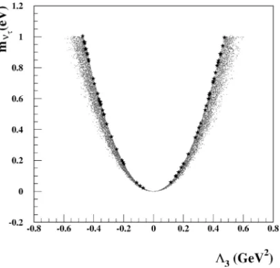
described by Eq. (37) with the replacement_| Λ_|2_→Λ2₃. In Fig. 6, we plot the neutrino mass as a function ofΛin AMSB-BRpV with the input parametersm3/2=32 TeV,µ <0, 5<tanβ <20, 100< m0<1000 GeV and 10−5< ǫ3<1 GeV. The quadratic dependence of the neutrino mass onΛis apparent in this figure and neutrino masses smaller than 1 eV occur for_|Λ_|0.6 GeV2. Moreover, the stars correspond to the allowed neutrino masses when the tau-sneutrino is the LSP. In general the points with a small (large)m0are located in the inner (outer) regions of this scattered plot.

From Fig. 6, we can see that the attainable neutrino masses are consistent with the global three-neutrino oscillation data analysis in the first reference of [10] that favors the

ντ→νµ oscillation hypothesis. Although only mass squared differences are constrained

by the neutrino data, our model naturally gives a hierarchical neutrino mass spectrum, therefore, we extract a naïve constraint on the actual mass coming from the analysis of the full atmospheric neutrino data, 0.04mντ 0.09 eV [10]. In addition, we notice that it

Fig. 6. Tau neutrino mass as a function ofΛ3for 5<tanβ <20, 100< m0<1000 GeV,m3/2=32 TeV and

Fig. 7. Mixing between CP-even Higgses and sneutrino as a function of the tau neutrino mass.

is not possible to find an upper bound on the neutrino mass if angular dependence on the neutrino data is not included and only the total event rates are considered.

In Fig. 7 we show the correlation between the neutrino mass and mixing of the tau-sneutrino and the CP-even Higgses (sinθeven) for the parameters assumed in Fig. 6. As expected, the largest mixings are associated to larger neutrino masses. Notwithstanding, it is possible to obtain large mixings for rather small neutrino masses because the mixing is proportional to theRP violating parametersǫ3andv3, and not directly onΛ3∝mντ. In any case, Fig. 7 suggests that large scalar mixings are still possible even imposing these bounds on the neutrino mass. This is extremely important for the phenomenology of the model because it indicates that non negligibleRP violating branching ratios are possible

for scalars even in the case they are not the LSP.

7. Discussions

The presence of RP violating interactions in our model render the LSP unstable,

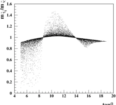
avoiding strong constraints on the possible LSP candidates. In the parameter regions where the neutralino is not the LSP, whether the light stau or the tau-sneutrino is the LSP depends crucially on the value of tanβ. This fact can be seen in Fig. 8 where we plot the ratio between the light stau and the tau-sneutrino masses as a function of tanβ

form3/2=32 TeV, 100< m0<300 GeV, andµ <0. From this figure we see that the tau-sneutrino is the LSP for 8.5tanβ14, otherwise the stau is the LSP.2

2 _{Of course,m}

Fig. 8. Ratio between the light stau and the sneutrino masses as a function of tanβ for m3/2=32 TeV, 100< m0<300 GeV andµ <0.

When the stau is the LSP, it decays viaRP violating interactions, i.e., its decays take

place through mixing with the charged Higgs, and consequently, they will mimic the charged Higgs boson ones. Therefore, it is very important to be able to distinguish between

˜

τ₁±andH±. This can be achieved either through precise studies of branching ratios, or via the mass spectrum, or both [21].

Measurements on the mass spectrum are also important in order to distinguish AMSB with and without conservation of RP. In Fig. 9 we present the ratio between the stau

mass splitting in AMSB-BRpV and in the AMSB,R₌(mτ_˜2−mτ˜1)AMSB−BRpV/(mτ˜2 −

mτ_˜1)AMSB, with ǫ3=v3=0 and keeping the rest of the parameters unchanged, as a function of tanβ. In these figures, we took 100< m0<1000 GeV,m3/2=32 TeV, and (a)µ >0, and (b)µ <0. Forµ >0 (Fig. 9(a)), the stau mass splitting is always larger in the AMSB-BRpV than in the AMSB by a factor that increases when tanβ decreases, and can be as large asR_∼10 for tanβ_∼3! We remind the reader that, in the absence ofRP

violation, the left–right stau mixing decreases with decreasing tanβ, thus augmenting the importance ofR-parity violating mixings. On the other hand, forµ <0 (Fig. 9(b)), this ratio can be as large as before at small tanβ, but in addition, the splitting can go to zero in AMSB-BRpV near tanβ_≈11, which also constitutes a sharp difference with the AMSB. For both signs ofµthe ratio goes to unity at large tanβ because the left–right mixing in the AMSB is proportional to tanβand dominates over anyRP violating contribution.

The behavior ofR at tanβ_∼11 in Fig. 9(b) indicates that the two staus can be nearly degenerated in AMSB-BRpV. In Fig. 10 we plot the ratio between the light and heavy stau masses as a function of tanβ, form3/2=32 TeV, 100< m0<300 GeV andµ <0, observing clearly that the near degeneracy occurs at tanβ_∼11. In first approximation, consider that the near degeneracy occurs whenAτvd−µvu≈0 as inferred from Eq. (27).

Fig. 9. Ratio (R) between the stau splitting in AMSB with and withoutRP violation as a function of tanβ, for:

m3/2=32 TeV, 100< m0<1000 GeV and (a)µ >0 or (b)µ <0.

in Eq. (38), which defines the atmospheric neutrino mass, as indicated in Eq. (37). The smallness of these two quantities implies that the mixingXuRin Eq. (31) is also small in

this particular region of parameter space, indicating that the right stau is decoupled from the Higgs fields and thus originating the zero in the mixing angle, noted already in Figs. 4 and 5.

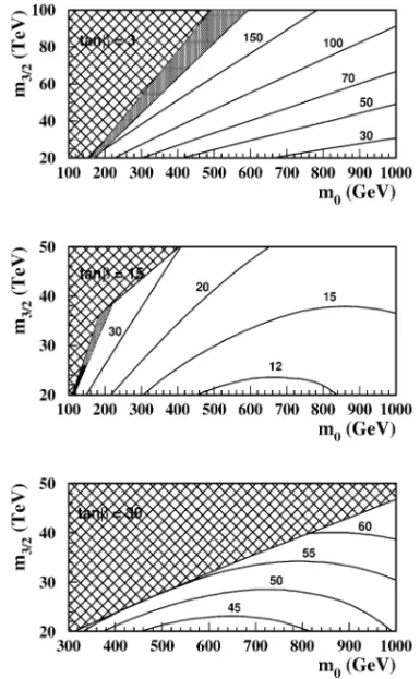
In order to quantify the stau mass splitting in our model, we present in Fig. 11 contours of constant splitting between the stau masses,mτ_˜2−mτ˜1, in the planem3/2×m0in GeV forµ <0 and several tanβ. We can see in Fig. 11(a) that for small tanβ ₌3 the stau mass splitting in our model starts atmτ_˜2 −mτ˜1 ∼30 GeV, in sharp contrast with theRP conserving case where the biggest splittings barely goes over this value [7]. This is in agreement with the results presented in Fig. 9(b). Furthermore, we can also see that there is a considerable region in them3/2×m0 plane, indicated by the grey area, where the

lightest stau is the LSP. For intermediary values of tanβ_∼15, Fig. 11(b) shows that the stau mass splitting goes to a minimum. This is a different behavior from the MSSM which presents a mass splitting up to 10 times bigger as we have seen in Fig. 9(b). For this value of tanβwe still have a small region where the lightest stau is the LSP (grey area) and, as a novelty, a tiny region for small values ofm3/2andm0where the tau-sneutrino is the LSP (black area). For large values of tanβ₌30, the stau splitting mass shown in Fig. 11(c) is similar to the MSSM one [7].

We have made below a series of three figures fixing the value tanβ₌15 to study the dependence onm0of the mass spectrum and mixings in the scalar sector. This choice of tanβ is such that we find a degeneracy among the masses, and consequently we obtain large mixings in the scalar sector. We also chosem3/2=32 TeV andµ <0, while theRP

violating parameters were varied according to 10−5< ǫ3<1 GeV and 10−6< mντ <1 eV. In Fig. 12(a) we plot tau-sneutrino mixing with the CP-odd neutral Higgs as a function ofm0for the parameters indicated above. We find quite large mixings form0≈320 GeV. In Fig. 12(b) we show the CP-odd Higgs and tau-sneutrino masses, which depend almost linearly onm0. Moreover, the value ofm0at which these two particles have the same mass coincides with the point of maximum mixing.

The CP-even tau-sneutrino mixing with the CP-even Higgs is presented in Fig. 13(a) as a function ofm0. There are two peaks of high mixing; the main one atm0≈320 GeV and

Fig. 13. (a) Mixing between the CP-even Higgs and sneutrino and (b) the light and heavy CP-even Higgs masses as well as the sneutrino one as a function ofm0form3/2=32 TeV,µ <0 and tanβ=15.

a narrow one atm0≈180 GeV. These two peaks have a different origin, as indicated by Fig. 13(b), where we plot the masses of the two CP-even neutral Higgs bosons,mhandmH,

and the mass of the CP-even tau-sneutrinomν_˜even

τ , as a function ofm0. We observe that the broad peak is due to a degeneracy between the tau-sneutrino and the heavy neutral Higgs boson and the narrow peak comes from a degeneracy between the tau-sneutrino and the light neutral Higgs boson. As expected, theH0andν_˜τevenmasses grow linearly withm0, contrary to theh0mass which remains almost constant.

In Fig. 14(a) we display the light stau mixing with the charged Higgs as a function of

m0. The maximum mixing, obtained atm0≈550 GeV, is the result of a mass degeneracy between the charged Higgs boson and the light stau. This can be observed in Fig. 14(b) where we plot the charged Higgs massmH± and the light stau mass mτ_˜1 as a function ofm0.

In a similar way, we show the heavy stau mixing with charged Higgs as a function of

Fig. 14. (a) Mixing of the charged Higgs with the light stau, (b) charged Higgs and light stau masses, (c) mixing of the charged Higgs with the heavy stau, and (d) charged Higgs and heavy stau masses as a function ofm0for

m3/2=32 TeV,µ <0 and tanβ=15.

As opposed to the scalar sector, where mixing between the Higgs bosons and sleptons can be maximum, in the chargino and neutralino sectors the mixings with leptons are controlled by the neutrino mass being very small. Despite this fact, the mixing in the neutralino sector is sufficient to generate adequate masses for the neutrinos and give rise to the neutralino decays mentioned in the introduction. Therefore, in the chargino sector the BRpV-AMSB phenomenology changes very little with respect to theRP conserving

AMSB. One of the distinctive features of AMSB that differentiates it from other scenarios of supersymmetry breaking in the chargino-neutralino sector is the near degeneracy between the lightest chargino and the lightest neutralino. This feature remains in BRpV-AMSB as was anticipated in Fig. 1. Form3/2=32 TeV,µ <0, and 100< m0<300 GeV, we show in Fig. 15 the lightest chargino mass as a function of tanβ. The lightest chargino mass has a small dependence on tanβsince its value varies only between 100 and 104 GeV. As inRP conserving AMSB, the mass differencem_χ˜+

Fig. 15. Light chargino mass as a function of tanβform3/2=32 TeV,µ <0 and 100< m0<300 GeV.

8. Conclusions

We have shown in the previous sections that our model exhibiting anomaly mediated supersymmetry breaking and bilinear RP violation is phenomenologically viable. In

particular, the inclusion of BRpV generates neutrino masses and mixings in a natural way. Moreover, theRP breaking terms give rise to mixing between the Higgs bosons and

the sleptons, which can be rather large despite the smallness of the parameters needed to generate realistic neutrino masses. These large mixings occur in regions of the parameter space where two states are nearly degenerate. Our model also alters substantially the mass splitting between the scalar taus in a large range of tanβ.

TheRP violating interactions render the LSP unstable since it can decay via its mixing

with the SM particles (leptons or scalars). Therefore, the constraints on the LSP are relaxed and forbidden regions of parameter space become allowed, where scalar particles like staus or sneutrinos are the LSP. Furthermore, the large mixing between Higgs bosons and sleptons has the potential to change the decays of these particles. These facts have a profound impact in the phenomenology of the model, changing drastically the signals at colliders [22].

Acknowledgements

Appendix A. AMSB boundary conditions

The AMSB boundary conditions at the GUT scale for the gaugino masses are proportional to their beta functions, resulting in

(A.1)

M1= 33

5

g2₁

16π2m3/2,

(A.2)

M2=

g₂2

16π2m3/2,

(A.3)

M3= −3

g₃2

16π2m3/2,

while the third generation scalar masses are given by

(A.4)

m2_{U =}

−₂₅88g₁4₊8g₃4₊2ftβˆft

0

m2_3/2

16π22₊m2₀,

(A.5)

m2_D=

−22

25g 4 1+8g

4

3+2fbβˆfb

_m2

3/2

(16π2₎2+m 2 0,

(A.6)

m2_Q=

−11₅₀g₁4₋3

2g 4

2+8g34+ftβˆft +fbβˆfb

_m2

3/2

(16π2₎2+m 2 0,

(A.7)

m2_L=

−99₅₀g₁4₋3

2g 4

2+fτβˆfτ

_m2

3/2

(16π2₎2+m 2 0,

(A.8)

m2_E=

−198₂₅ g4₁₊2fτβˆfτ

_m2

3/2

(16π2₎2+m 2 0,

(A.9)

m2_H

u=

−99₅₀g₁4₋3

2g 4

2+3ftβˆft

_m2

3/2

(16π2₎2+m 2 0,

(A.10)

m2_H

d =

−99₅₀g₁4₋3

2g 4

2+3fbβˆfb+fτβˆfτ

_m2

3/2

(16π2₎2+m 2 0. Finally, theA-parameters are given by

(A.11)

At=

ˆ

βft

ft

m3/2

16π2, Ab=

ˆ

βfb

fb

m3/2

16π2, Aτ=

ˆ

βfτ

fτ

m3/2 16π2, where we have defined

(A.12)

ˆ

βft=16π 2_β

t=ft

−13₁₅g₁2₋3g2₂₋16

3 g 2

3+6ft2+fb2

,

(A.13)

ˆ

βfb=16π 2_β

b=fb

−₁₅7 g2₁₋3g₂2₋16

3 g 2 3+f

2

t +6f

2

b +f

2 τ , (A.14) ˆ

βfτ=16π 2_β

τ=fτ

−9₅g2₁₋3g₂2₊3f_b2₊4f_τ2

Appendix B. The renormalization group equations

Here we present the one-loop renormalization group equations for our model, assuming the bilinearRP breaking terms are restricted only to the third generation. First, we display

the equations for the Yukawa couplings of the trilinear terms

(B.1) 16π2dhU

dt =hU

6h2_U+h2_D−16

3 g 2 3−3g

2 2− 13 9 g 2 1 , (B.2) 16π2dhD

dt =hD

6h2_D+h2_U+h2_τ−16

3 g 2

3−3g22− 7 9g 2 1 , (B.3) 16π2dhτ

dt =hτ

4h2_τ+3h2_D−3g₂2₋3g2₁

.

The corresponding RGE for cubic soft supersymmetry breaking parameters are given by

(B.4) 8π2dAU

dt =6h

2

UAU+h2DAD+

16 3 g

2

3M3+3g22M2+ 13

9 g 2 1M1,

(B.5) 8π2dAD

dt =6h

2

DAD+h2UAU+h2τAτ+

16 3 g

2

3M3+3g22M2+ 7 9g

2 1M1,

(B.6) 8π2dAτ

dt =4h

2

τAτ+3h2DAD+3g22M2+3g21M1. For the soft supersymmetry breaking mass parameters we have

(B.7) 8π2dM

2

Q

dt =h

2

U

m2_H

2+M 2

Q+MU2 +A2U

+h2_Dm2_H

1+M 2

Q+MD2 +A2D

−16₃ g₃2M₃2₋3g₂2M₂2₋1

9g 2 1M12+

1 6 g

2 1S, 8π2dM

2

U

dt =2h

2

U

m2_H

2+M 2

Q+MU2 +A2U

−16₃ g₃2M₃2₋16

9 g 2 1M12−

2 3 g

2 1S,

(B.8)

(B.9) 8π2dM

2

D

dt =2h

2

D

m2_H

1+M 2

Q+MD2 +A2D

−16₃ g₃2M₃2₋4

9g 2 1M 2 1+ 1 3 g 2 1S,

(B.10) 8π2dM

2

L

dt =h

2

τ

m2_H

1+M 2

L+MR2+A2τ

−3g2₂M₂2₋g₁2M₁2₋1

2 g 2 1S,

(B.11) 8π2dM

2

R

dt =2h

2

τ

m2_H

1+M 2

L+M

2

R+A

2

τ

−4g2₁M₁2₊g₁2S,

(B.12) 8π2dm

2

H2

dt =3h

2

U

m2_H

2+M 2

Q+MU2 +A2U

−3g₂2M₂2₋g2₁M₁2₊1

2 g 2 1S,

(B.13) 8π2dm

2

H1

dt =3h

2

D

m2_H

1+M 2

Q+MD2+A2D

+h2_τm2_H

1+M 2

L+MR2+A2τ

−3g₂2M₂2₋g₁2M₁2₋1

2 g 2 1S, where

(B.14) S₌m2_H

2−m 2

H1+M 2

Q−2M

2

U+M

2

D−M

2

L+M

2

For the bilinear terms in the superpotential we get

(B.15) 16π2dµ

dt =µ

3h2_U+3h2_D+h_τ2₋3g2₂₋g₁2,

(B.16) 16π2dǫ3

dt =ǫ3

3h2_U+h2_τ−3g2₂₋g2₁,

and for the corresponding soft breaking terms

(B.17) 8π2dB

dt =3h

2

UAU+3h2DAD+h2τAτ+3g22M2+g12M1,

(B.18) 8π2dB2

dt =3h

2

UAU+h2τAτ+3g22M2+g21M1.

Thegi are the SU(3)×SU(2)×U (1)gauge couplings and theMi are the corresponding

soft breaking gaugino masses.

References

[1] A. Chamseddine, R. Arnowitt, P. Nath, Phys. Rev. Lett. 49 (1982) 970; R. Barbieri, S. Ferrara, C. Savoy, Phys. Lett. B 119 (1982) 343; L.J. Hall, J. Lykken, S. Weinberg, Phys. Rev. D 27 (1983) 2359. [2] M. Dine, A. Nelson, Phys. Rev. D 48 (1993) 1277;

M. Dine, A. Nelson, Y. Shirman, Phys. Rev. D 51 (1995) 1362; M. Dine, A. Nelson, Y. Nir, Y. Shirman, Phys. Rev. D 53 (1996) 2658. [3] L. Randall, R. Sundrum, Nucl. Phys. B 557 (1999) 79;

G. Giudice, M. Luty, H. Murayama, R. Rattazzi, JHEP 9812 (1998) 027. [4] T. Gherghetta, G.F. Giudice, J.D. Wells, Nucl. Phys. B 559 (1999) 27. [5] A. Pomarol, R. Rattazzi, JHEP 9905 (1999) 013;

Z. Chacko, M.A. Luty, I. Maksymyk, E. Ponton, JHEP 0004 (2000) 001; E. Katz, Y. Shadmi, Y. Shirman, JHEP 9908 (1999) 015;

M.A. Luty, R. Sundrum, Phys. Rev. D 62 (2000) 035008; J.A. Bagger, T. Moroi, E. Poppitz, JHEP 0004 (2000) 009; I. Jack, D.R.T. Jones, Phys. Lett. B 482 (2000) 167;

M. Kawasaki, T. Watari, T. Yanagida, Phys. Rev. D 63 (2001) 083510. [6] T. Moroi, L. Randall, Nucl. Phys. B 570 (2000) 455;

G.D. Kribs, Phys. Rev. D 62 (2000) 015008; S. Su, Nucl. Phys. B 573 (2000) 87;

R. Rattazzi, A. Strumia, J.D. Wells, Nucl. Phys. B 576 (2000) 3; M. Carena, K. Huitu, T. Kobayashi, Nucl. Phys. B 592 (2001) 164; H. Baer, M.A. Díaz, P. Quintana, X. Tata, JHEP 0004 (2000) 016; D.K. Ghosh, P. Roy, S. Roy, JHEP 0008 (2000) 031;

U. Chattopadhyay, D.K. Ghosh, S. Roy, Phys. Rev. D 62 (2000) 115001; H. Baer, J.K. Mizukoshi, X. Tata, Phys. Lett. B 488 (2000) 367. [7] J.L. Feng, T. Moroi, Phys. Rev. D 61 (2000) 095004.

[8] B.C. Allanach, A. Dedes, JHEP 0006 (2000) 017. [9] B. Allanach et al., hep-ph/9906224;

B. Allanach et al., J. Phys. G 24 (1998) 421.

[10] M.C. Gonzalez-García, M. Maltoni, C. Peña-Garay, J.W.F. Valle, Phys. Rev. D 63 (2001) 033005; J.N. Bahcall, P.I. Krastev, A.Yu. Smirnov, JHEP 0105 (2001) 015.

[12] F. de Campos, O.J.P. Éboli, M.A. García-Jareño, J.W.F. Valle, Nucl. Phys. B 546 (1999) 33; R. Kitano, K. Oda, Phys. Rev. D 61 (2000) 113001;

D.E. Kaplan, A.E. Nelson, JHEP 0001 (2000) 033; C.-H. Chang, T.-F. Feng, Eur. Phys. J. C 12 (2000) 137; M. Frank, Phys. Rev. D 62 (2000) 015006;

F. Takayama, M. Yamaguchi, Phys. Lett. B 476 (2000) 116; K. Choi, E.J. Chun, K. Hwang, Phys. Lett. B 488 (2000) 145;

J.M. Mira, E. Nardi, D.A. Restrepo, J.W.F. Valle, Phys. Lett. B 492 (2000) 81. [13] R. Hempfling, Nucl. Phys. B 478 (1996) 3.

[14] J.C. Romão, M.A. Díaz, M. Hirsch, W. Porod, J.W.F. Valle, Phys. Rev. D 61 (2000) 071703; M. Hirsch, M.A. Díaz, W. Porod, J.C. Romão, J.W.F. Valle, Phys. Rev. D 62 (2000) 113008. [15] T. Banks, Y. Grossman, E. Nardi, Y. Nir, Phys. Rev. D 52 (1995) 5319;

A.S. Joshipura, M. Nowakowski, Phys. Rev. D 51 (1995) 2421;

G. Bhattacharyya, D. Choudhury, K. Sridhar, Phys. Lett. B 349 (1995) 118; M. Nowakowski, A. Pilaftsis, Nucl. Phys. B 461 (1996) 19;

A.Yu. Smirnov, F. Vissani, Nucl. Phys. B 460 (1996) 37;

J.C. Romão, F. de Campos, M.A. García-Jareño, M.B. Magro, J.W.F. Valle, Nucl. Phys. B 482 (1996) 3; B. de Carlos, P.L. White, Phys. Rev. D 54 (1996) 3427;

B. de Carlos, P.L. White, Phys. Rev. D 55 (1997) 4222; H. Nilles, N. Polonsky, Nucl. Phys. B 484 (1997) 33. [16] A. Santamaria, J.W.F. Valle, Phys. Lett. B 195 (1987) 423;

A. Santamaria, J.W.F. Valle, Phys. Rev. Lett. 60 (1988) 397; A. Santamaria, J.W.F. Valle, Phys. Rev. D 39 (1989) 1780. [17] M.A. Díaz, J.C. Romão, J.W.F. Valle, Nucl. Phys. B 524 (1998) 23.

[18] A. Akeroyd, M.A. Díaz, J. Ferrandis, M.A. García-Jareño, J.W.F. Valle, Nucl. Phys. B 529 (1998) 3; M.A. Díaz, J. Ferrandis, J.C. Romão, J.W.F. Valle, Phys. Lett. B 453 (1999) 263;

A.G. Akeroyd, M.A. Díaz, J.W.F. Valle, Phys. Lett. B 441 (1998) 224; M.A. Díaz, E. Torrente-Lujan, J.W.F. Valle, Nucl. Phys. B 551 (1999) 78; M.A. Díaz, J. Ferrandis, J.C. Romão, J.W.F. Valle, Nucl. Phys. B 590 (2000) 3; M.A. Díaz, D.A. Restrepo, J.W.F. Valle, Nucl. Phys. B 583 (2000) 182; M.A. Díaz, J. Ferrandis, J.W.F. Valle, Nucl. Phys. B 573 (2000) 75. [19] M. Frank, K. Huitu, Phys. Rev. D 64 (2001) 095015.

[20] M.A. Díaz, hep-ph/9802407.