www.clim-past.net/7/1415/2011/ doi:10.5194/cp-7-1415-2011
© Author(s) 2011. CC Attribution 3.0 License.
of the Past
The role of orbital forcing, carbon dioxide and regolith
in 100 kyr glacial cycles
A. Ganopolski and R. Calov
Potsdam Institute for Climate Impact Research, Potsdam, Germany Received: 24 June 2011 – Published in Clim. Past Discuss.: 18 July 2011
Revised: 27 October 2011 – Accepted: 28 October 2011 – Published: 14 December 2011
Abstract. The origin of the 100 kyr cyclicity, which dom-inates ice volume variations and other climate records over the past million years, remains debatable. Here, using a com-prehensive Earth system model of intermediate complexity, we demonstrate that both strong 100 kyr periodicity in the ice volume variations and the timing of glacial terminations during past 800 kyr can be successfully simulated as direct, strongly nonlinear responses of the climate-cryosphere sys-tem to orbital forcing alone, if the atmospheric CO2
con-centration stays below its typical interglacial value. The ex-istence of long glacial cycles is primarily attributed to the North American ice sheet and requires the presence of a large continental area with exposed rocks. We show that the sharp, 100 kyr peak in the power spectrum of ice volume re-sults from the long glacial cycles being synchronized with the Earth’s orbital eccentricity. Although 100 kyr cyclicity can be simulated with a constant CO2concentration,
tempo-ral variability in the CO2 concentration plays an important
role in the amplification of the 100 kyr cycles.
1 Introduction
Although it is generally accepted that, as postulated by the Milankovitch theory (Milankovitch, 1941), Earth’s orbital variations play an important role in Quaternary climate dy-namics, the nature of glacial cycles still remains poorly un-derstood. One of the major challenges to the classical Mi-lankovitch theory is the presence of 100 kyr cycles that dom-inate global ice volume and climate variability over the past million years (Hays et al., 1976; Imbrie et al., 1993; Paillard, 2001). This periodicity is practically absent in the princi-pal “Milankovitch forcing” – variations of summer insolation
Correspondence to:A. Ganopolski ([email protected])
at high latitudes of the Northern Hemisphere (NH). The ec-centricity of Earth’s orbit does contain periodicities close to 100 kyr and the robust phase relationship between glacial cy-cles and 100-kyr eccentricity cycy-cles has been found in the paleoclimate records (Hays et al., 1976; Berger et al., 2005; Lisiecki, 2010). However, the direct effect of the eccentric-ity on Earth’s global energy balance is very small. More-over, eccentricity variations are dominated by a 400 kyr cycle which is also seen in some older geological records (e.g. Za-chos et al., 1997), but is practically absent in the frequency spectrum of the ice volume variations for the last million years. In view of this long-standing problem, it was pro-posed that the 100 kyr cycles do not originate directly from the orbital forcing but rather represent internal oscillations in the climate-cryosphere (Gildor and Tziperman, 2001) or climate-cryosphere-carbonosphere system (e.g. Saltzman and Maasch, 1988; Paillard and Parrenin, 2004), which can be synchronized (phase locked) to the orbital forcing (Tziperman et al., 2006). Alternatively, it was proposed that the 100 kyr cycles result from the terminations of ice sheet buildup by each second or third obliquity cycle (Huybers and Wunsch, 2005) or each fourth or fifth precessional cy-cle (Ridgwell et al., 1999) or they originate directly from a strong, nonlinear, climate-cryosphere system response to a combination of precessional and obliquity components of the orbital forcing (Paillard, 1998). Since a number of concep-tual models based on fundamentally different assumptions were able to reproduce reconstructed ice volume variations with similar skill, it became clear that a further advance in understanding of 100 kyr cyclicity requires physically-based models.
and were additionally accompanied by pronounced variabil-ity at another eccentricvariabil-ity frequency – 400 kyr – which is not seen in the spectra of reconstructed ice volume. It was only when realistic CO2forcing was applied in addition to orbital
forcing that realistic simulations of the glacial cycles became possible (Berger et al., 1998). The notable exception is the work by Pollard (1983) wherein after adding several non-linear process, the model forced by orbital variations alone simulates strong 100 kyr cycles in agreement with the ice volume reconstructions available at that time. It is interest-ing to note that the agreement is even more impressive when Pollard’s modelling results are compared to the most recent reconstructions of ice volume.
Although simplified climate-cryosphere models demon-strate the possibility of the appearance of the 100 kyr cycle as a direct response of the climate-cryosphere system to the orbital forcing, due to their simplicity (usually these mod-els were based on a one-dimensional ice sheet model and an energy balance atmosphere model), doubt remains whether these results are fully applicable to the real world. Moover, the presence of 400 kyr cycles in many simulations re-mains an obvious problem. Therefore, it is crucial to corrob-orate earlier results and further advance the understanding of glacial cycles by using more physically based and geograph-ically explicit climate-cryosphere models. While coupled GCMs still remain too expensive for simulating glacial cy-cles, models of intermediate complexity (EMICs, Claussen et al., 2002) can be coupled to 3-D ice sheet models and are sufficiently computationally efficient to perform simula-tions of glacial cycles. Using CLIMBER-2 coupled to dif-ferent ice sheet models, Bonelli et al. (2009) and Ganopol-ski et al. (2010) performed simulations of the last glacial cycles; Calov and Ganopolski (2005) analysed the stabil-ity of the climate-cryosphere system in the phase space of Milankovitch forcing and Bauer and Ganopolski (2010) re-ported simulations of the last four glacial cycles. Here we will present a large suite of simulations for the last 800 kyr, a period of time dominated by 100 kyr cyclicity.
2 Model description and experimental setup
The model used in the study is the most recent version of the Earth system model of intermediate complexity CLIMBER-2 (Petoukhov et al., CLIMBER-2000; Ganopolski et al., CLIMBER-2001; Brovkin et al., 2002), which includes a 3-D polythermal ice sheet model (Greve, 1997). The ice sheet model is only applied to the Northern Hemisphere and is coupled to the climate compo-nent via a high-resolution, physically-based surface energy and mass balance interface (Calov et al., 2005), which ex-plicitly accounts for the effect of aeolian dust deposition on snow albedo. Here we use the same model and experimental setup as Ganopolski et al. (2010) but extended it to simulate glacial cycles over the past 800 000 years.
In all experiments the equilibrium state of the climate-cryosphere system obtained for present-day conditions was used as the initial condition and the model was run from 860 kyr BP until the present. The first 60 000 years, repre-senting the model spin-up, were not used for further analysis. In the Baseline Experiment (referred to hereafter as BE), we prescribed variations in orbital parameters following Berger (1978) and the equivalent CO2concentration, which
accounts for the radiative forcing of three major greenhouse gases – carbon dioxide, methane and nitrous oxide. Their concentrations were derived from the Antarctic ice cores (Pe-tit et al., 1999; EPICA, 2004). The method used to calculate the equivalent CO2 concentration is described by
Ganopol-ski et al. (2010). A continuous record of N2O is not
avail-able for the last 800 kyr, but existing data suggest that, to the first approximation, the N2O concentration has a
tempo-ral dynamic similar to CO2. Therefore, we assumed that the
radiative forcing of N2O (relative to preindustrial) is 20 % of
that of CO2during the whole simulated period, i.e. the ratio
between radiative forcings of N2O and CO2is the same as at
the LGM.
Although concentrations of GHGs from the ice cores are only available for the last 800 000 years, the time 800 kyr BP is not the best choice for the beginning of the simulations be-cause it was close to a glacial maximum and therefore would require an initialization of the large continental ice sheets in the Northern Hemisphere. For this reason, we begin our sim-ulations at 860 kyr BP, which corresponds to the MIS 21 in-terglacial for which we can use the equilibrium present-day climate state as initial conditions. However, this choice of the initial state requires prescription of the equivalent CO2
concentration for the time interval when reliable data for GHGs concentration are not yet available. To extend the time series of equivalent CO2 concentration beyond 800 kyr BP,
we made use of a close correlation between the total radia-tive forcing of GHGs and benthicδ18Ocstack (Lisiecki and
Raymo, 2005) observed for the last 800 kyr. By using a sim-ple linear regression, we calculated equivalent CO2
concen-tration for these initial 60 kyr. Since this period was con-sidered as the model spin-up and was not used for further analysis, the accuracy of this reconstruction of the equivalent CO2is not crucial for the results presented in the paper.
In addition to the BE, we performed a large suite of exper-iments with constant CO2, modified orbital forcing, and
ter-restrial sediment mask. These experiments are summarized in Table 1.
3 Results
3.1 Baseline experiment
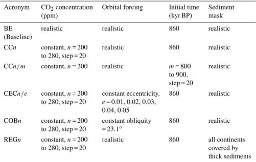
Table 1.List of model experiments.
Acronym CO2concentration Orbital forcing Initial time Sediment
(ppm) (kyr BP) mask
BE realistic realistic 860 realistic (Baseline)
CCn constant,n= 200 realistic 860 realistic to 280, step = 20
CCn/m constant,n= 200 realistic m= 800 realistic to 900,
step = 20
CECn/e constant,n= 200 constant eccentricity, 860 realistic to 280, step = 20 e= 0.01, 0.02, 0.03,
0.04, 0.05
COBn constant,n= 200 constant obliquity 860 realistic to 280, step = 20 = 23.1◦
REGn constant,n= 200 realistic 860 all continents to 280, step = 20 covered by
thick sediments
Fig. 1. (a) Maximum summer insolation at 65◦N; (b)
radia-tive forcing of prescribed equivalent CO2concentration;(c)
sim-ulated (green) versus reconstructed (grey) Greenland temperature anomaly;(d)simulated (orange) versus reconstructed (grey) tropi-cal SST anomaly,(e)simulated (blue) versus reconstructed (grey) Antarctic temperature anomaly.
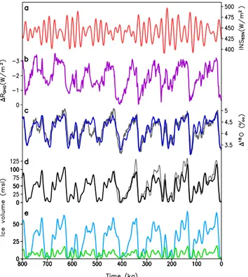
Fig. 2. (a)Maximum summer insolation at 65◦N; (b) radiative
forcing of prescribed equivalent CO2concentration;(c)simulated (blue) versus reconstructed (grey) benthicδ18Ocstack (Lisiecki and
Raymo, 2005),(d) simulated (black) versus reconstructed (grey) global sea level change (Waelbroeck et al., 2002); (e)simulated North American (blue) and European (green) ice volume in meters of sea level (m.s.l.).
cooling compared to empirical data during MIS 6 and 16 is difficult to explain.
Figure 2 shows that the model successfully simulates the waxing and waning of the ice sheets with a dominant 100 kyr periodicity and a pronounced asymmetry of the glacial cy-cles. For the second half of the run (Fig. 2d), modeling re-sults agree favorably with reconstructed variations of global sea level by Waelbroeck et al. (2002). For the earlier part of the modeled period, reliable reconstructions of global ice volume are lacking, and the benthicδ18Ocstack by Lisiecki
and Raymo (2005) was used for comparison. Since benthic δ18Ocis not an accurate proxy for ice volume, we computed
the model’s equivalent ofδ18Ocfrom the simulated global ice
volume and deep ocean temperature using a simple relation-ship between the three (Duplessy et al., 1991). In addition, based on the results of simulations of the Antarctic ice sheet evolution during the last glacial cycle (Huybrechts, 2002), we assume that the Southern Hemisphere contributed an ad-ditional 10 % to global ice volume variations. Computed in this way, the modelled δ18Oc agrees reasonably well with
the empirical benthicδ18Ocstack (Fig. 2c). It is also not
sur-prising that the agreement is better for the second part of the model run than for the first one (prior to MIS 11). Indeed,
Fig. 3. (a)Frequency spectrum of the simulated (black) versus re-constructed (grey) benthicδ18Ocstack (Lisiecki and Raymo, 2005);
(b)–(f)frequency spectra of the simulated ice volume:(b)Baseline experiment,(c)CCnexperiments with constant CO2,(d)COBn
ex-periments with constant obliquity,(e)CECn/0.02 experiments with constant (0.02) eccentricity,(f)REGnexperiments with continents completely covered by sediments. In (c)–(f), purple lines corre-spond to a CO2concentration of 200 ppm, blue – 220 ppm, green –
240 ppm, orange – 260 ppm and red – 280 ppm.
the model used in this study was tuned for the last glacial cycles and, since several previous cycles resemble the last one in many respects, it is not surprising that the model re-sults compare well with the proxy data also for these cycles. However, prior to MIS 11, the magnitude ofδ18Ocand CO2
variations was smaller, which is likely due to difference in the Earth’s topography and/or sediment distribution, which gradually evolved over geological time scales. Since these changes were not taken into account, degrading of the model agreement with the data further into the past is natural. The largest discrepancy between simulated and empiricalδ18Oc
stack occurs during MIS 14 (ca. 550 ka). Whether this is an indication of model deficiencies or dating problems of the proxy records is not clear.
The frequency spectra of modeled and empiricalδ18Ocare
also in good agreement (Fig. 3a). All three major peaks – 100, 41 and 23 kyr are reproduced with the dominance of 100 kyr cycle and a weaker precessional cycle, even though the modeledδ18Occontains more spectral power in the
Figure 2e shows the simulated volume of the North Ameri-can and Eurasian ice sheets. Similarly to the last glacial cycle (Ganopolski et al., 2010), the global ice volume is dominated by the North American ice sheet, which agrees with Bintanja and van de Wal (2008). It also has stronger 100 kyr cyclic-ity whilst the Eurasian ice sheet reveals more variabilcyclic-ity at the precessional time scale. Simulated maxima in ice vol-ume and ice area (not shown) are rather similar for both ice sheets for the LGM and penultimate glacial maximum. This is explained by the fact that the history and the magnitude of the orbital and GHG forcings prior to both glacial maxima were rather similar and, as a result, the simulated temperature over the NH continents at the end of MIS 6 and MIS 2 are rather similar as well. At the same time, paleoclimate recon-structions suggest (Svendsen et al., 2004) that the maximum extent of the Eurasian ice sheet in Russia and Siberia during the penultimate glaciation was significantly larger than at the LGM. This implies that our model underestimates the sensi-tivity of the Eurasian ice sheet area to the orbital forcings. In particular, it is possible that the background dust deposition taken from GCM simulations for the LGM (Mahowald et al., 2006) is too high over this area, which restricts the eastward advance of the Eurasian ice sheet, thus making its area less sensitive to climate forcing than it is in reality. In the future, we are planning to avoid this problem by using a fully in-teractive dust model instead of the prescribed GCM output (Bauer and Ganopolski, 2010).
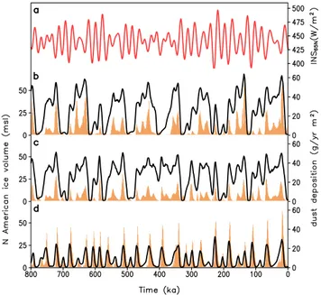
As discussed by Ganopolski et al. (2010), both the magni-tude and temporal dynamics of the simulated glacial cycles are very sensitive to the choice of model parameters, in par-ticular, related to surface mass balance, basal sliding, and glaciogenic dust. It was also shown that without enhanced dust deposition, complete deglaciation is not achieved in the model. Figure 4b shows the simulated dust deposition rate over the southern margin of the North American ice sheet. Each glacial termination is associated with a large increase in dust deposition, which reduces surface albedo and enhances ablation. There are two main reasons for the increase in the dust deposition rate during glacial termination: (i) a consid-erable portion of the North American ice sheet at the glacial maxima spreads over the area covered by thick terrestrial sediments and (ii) most of the ice sheet base over this area is at the pressure melting point. Both of these factors en-able fast sliding of the ice sheets and a large sediment trans-port towards the ice margins which, in turn, lead to enhanced glaciogenic dust production and dust deposition over the ice sheets. This amplifies the direct effect of rising summer in-solation and GHGs concentration.
The realistic simulation of climate-cryosphere dynamics over past 800 kyr in the BE performed with prescribed or-bital and GHG forcings represents an important test for the model. However, such an experiment does not answer the question about the origin of the strong 100 kyr cycles, since it is possible that the dominant 100 kyr periodicity and the correct timing of glacial terminations are solely attributed to
Fig. 4. (a)Maximum summer insolation at 65◦N; (b)simulated
volume of the North American ice sheet in msl (black line) and dust deposition rate (orange) at the southern margin of the ice sheet in the Baseline experiment,(c)the same as(b)but for the CC200 experiment,(d)the same as(b)but for REG200 experiment. The dust deposition rate is sampled at the location (45◦N, 100◦E).
the prescribed GHG forcing, the temporal dynamics of which strongly resembles the ice volume.
3.2 Experiments with constant CO2
To clarify whether the 100 kyr cycles directly originate from the orbital forcing, we performed a set of additional experi-ments (referred to hereafter as CCn, wherenis the prescribed CO2concentration in ppm, also see Table 1) with the same
orbital forcing as in the BE described above but maintaining a constant CO2concentration in time. We performed five
ex-periments with the CO2concentration ranging from 200 to
280 ppm (for every 20 ppm). Figure 5a shows a representa-tive subset of these simulations, while Fig. 6a shows the re-sults of all CCnexperiments for the whole range of CO2
con-centrations from 200 to 280 ppm. Quasi-regular glacial cy-cles are simulated for all CO2concentrations, with the
mag-nitude of the ice volume variations increasing for decreas-ing CO2. For a CO2 concentration of 280 ppm, simulated
glacial cycles are dominated by obliquity and precession, but for lower CO2concentrations, the model simulates long and
Fig. 5. Simulated ice volume variations in a subset of the exper-iments with constant CO2 (colored lines) versus the Baseline
ex-periment (grey shading). (a)CCnexperiments,(b)COBn exper-iments (constant obliquity),(c)CECn/0.02 experiments (constant eccentricity equal to 0.02),(d)REGnexperiments (with continents completely covered by thick sediment layer). Black lines corre-spond to a CO2concentration of 200 ppm, blue – 220 ppm and red
– 280 ppm. Dashed line at the top shows eccentricity.
indicates a direct relationship of the long glacial cycles with eccentricity variations. Unlike (Crowley and Hyde, 2008) who found the existence of 100 kyr cycles in a narrow range of CO2 concentrations, in our simulations 100 kyr cycles
are robust over a broad range of CO2concentrations (200–
260 ppm).
It is important to note that in the simulations with a con-stant CO2concentration below 260 ppm, not only the ice
vol-ume changes are dominated by the 100 kyr cycles, but simu-lated glacial terminations also occur at the same time as in the experiment with prescribed time-dependent CO2and, within
the dating accuracy, are in good agreement with paleoclimate reconstructions. The only exception is for MIS 11 (around 400 kyr BP), when complete deglaciation of the Northern Hemisphere does not occur in the experiments with low CO2
concentrations. The latter fact is not surprising since the or-bital forcing was weak during MIS 11 due to low eccentricity. Whether this problem implies that for this specific termina-tion the role of CO2is more important than for the others or
that the model is still not sufficiently non-linear to remove the ice under MIS 11 orbital forcing cannot be answered within the context of this study.
Although 860 kyr BP represents a convenient time to start simulations of the last glacial cycles, since it corresponds to an interglacial state and therefore does not require initialisa-tion of the continental ice sheets, it is theoretically possible
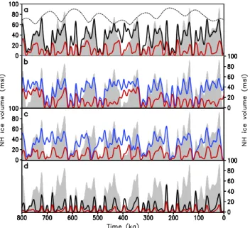
Fig. 6. Robustness of simulated glacial cycles. (a)Simulated NH ice volume variations in the experiments CCn(constant CO2). The colours indicate the CO2levels: 200 ppm (black), 220 ppm (blue),
240 ppm (green), 260 ppm (orange), 280 ppm (red). (b)Simulated NH ice volume variations in the experiments CC200/m starting from identical (interglacial) initial conditions but at a different time:
m= 900 kyr BP (purple),m= 880 kyr BP (orange),m= 860 (black),
m= 840 (light blue),m= 820 (green) andm= 800 (violet) kyr BP.
(c)Simulated NH ice volume variations in experiment CC200 with the standard glaciogenic parameterization (black), doubled (red) and halved (blue) glaciogenic dust deposition rate.
that this choice can be crucial for the timing of simulated glacial terminations and therefore a good agreement between simulated and real glacial terminations would be accidental. To show that this is not the case and that the timing of the glacial terminations is solely controlled by the orbital forc-ing, we performed an additional set of model simulations for constant CO2concentration equal to 200 ppm, where we
gan the model runs at the different astronomical times be-tween 800 and 900 kyr BP using the same (interglacial) initial conditions. These experiments are referred to as CC200/m, wheremdenotes the timing of the start of the experiment. Figure 6b shows that in all CC200/mexperiments the sim-ulated ice volume converged within one glacial cycle to the same solution. Therefore, the temporal dynamics and tim-ings of glacial terminations after the model spin-up are not sensitive to the choice of the beginning of the models runs.
As was shown by Ganopolski et al. (2010), simulation of a complete glacial termination, even with the prescribed GHG forcing, is only possible when the deposition of glacio-genic dust is taken into account. This is even more impor-tant in the case of a consimpor-tant CO2 concentration. Without
glaciogenic dust, long glacial cycles are not simulated in our model. Similarly to the BE, in the experiments with constant CO2(Fig. 4c), the rate of dust deposition over the southern
simulated glacial cycles over the entire 800 kyr period are rather sensitive to the poorly constrained parameters of the dust deposition scheme. Nonetheless, Fig. 6c shows that both doubling and halving of the glaciogenic dust deposition rate does not change the dominant 100 kyr cyclicity or the timing of major glacial terminations. Therefore, although details of the simulated glacial cycles depend on the dust parameteri-zation, the simulated 100 kyr cyclicity is robust with respect to the strength of the dust feedback.
3.3 Sensitivity of glacial cycles to different components of the orbital forcing
To find which component of the orbital forcing is respon-sible for the existence of 100 kyr cyclicity, we performed a suite of additional experiments in which, similar to the CCn set, the CO2concentration was held constant but the orbital
forcing was modified. In the first set of experiments (re-ferred as COBn), we removed the effect of obliquity varia-tions by setting obliquity constant in time and equal to its av-erage value over the simulated period (Fig. 7b). As shown in Fig. 5b, the removal of obliquity variations does not qualita-tively affect the simulated glacial cycles. For sufficiently low CO2 concentrations, long glacial cycles with a sharp
maxi-mum in the frequency spectra at 100 kyr periodicity are sim-ulated (Fig. 3d). However, fixing obliquity results in a nar-rower range of CO2concentrations for which 100 kyr
cyclic-ity dominates the frequency spectra. In addition, fixing obliq-uity makes glacial terminations less robust for the periods of low eccentricity, particularly during the most recent ter-mination. At the same time, all terminations that occurred during high eccentricity are correctly simulated in the COBn experiments.
In the complimentary set of experiments (referred to as CECn/e), we modified the orbital forcing by setting eccen-tricity constant in time with a value in the range 0–0.05, which covers real variations of eccentricity (Fig. 7c). Varia-tions of obliquity and precession were the same as in reality. For eccentricity lower than 0.02, the model failed to simu-late pronounced glacial cycles and for eccentricity of 0.04 and higher, the ice volume variations are dominated by pre-cession (not shown). However, for intermediate values of eccentricity (0.02 and 0.03) and sufficiently low CO2
con-centrations, the model simulates long glacial cycles (Fig. 5c). Moreover, many (but not all) simulated glacial terminations occur in the CEC220/0.02 experiments at the right time. However, the frequency spectra of ice volume variations in CECn/eexperiments lack a sharp peak in the 100 kyr band (Fig. 3e). In fact, the shape of the frequency spectrum in these experiments is very sensitive to the CO2level and the
maximum of spectral power tends to occur at one or multi-ples of obliquity periods, rather than at 100 kyr. Therefore, in our experiments obliquity variations themselves are not re-sponsible for the existence of the 100 kyr cycles, but they do contribute to the robustness of the long glacial cycles. It is
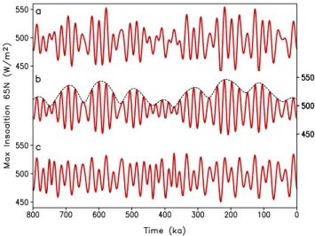
Fig. 7. Maximum summer insolation at 65◦N in(a)the BE, CCn
and REGnexperiments,(b)the experiment with constant obliquity (COBn) and(c)constant eccentricity (e= 0.02, CECn/0.02). The dashed line in panel(b)shows the amplitude modulation of the pre-cessional cycle by eccentricity.
noteworthy that the experiments described above essentially repeat the work by Pollard (1983). Although the principal mechanism of glacial terminations is different in our and in Pollard’s models, the main results are very similar.
3.4 The role of regolith
To gain insight into the possible origin of the mid-Pleistocene transition (around 1 million years ago), when the dominant periodicity of the glacial cycles changed from 40 kyr to 100 kyr (Ruddiman et al., 1989), we performed a set of model experiments identical to the CCnset, except for the spatial distribution of terrestrial sediments. We prescribed namely the presence of a thick terrestrial sediment layer for all conti-nental grid cells, while in the previous experiments we used a realistic distribution of terrestrial sediments. This set of ex-periments is referred to as REGn. With the continents com-pletely covered by sediments, the 100 kyr cyclicity is absent in the simulated ice volume for the whole range of prescribed CO2 concentrations and the ice volume variations are of a
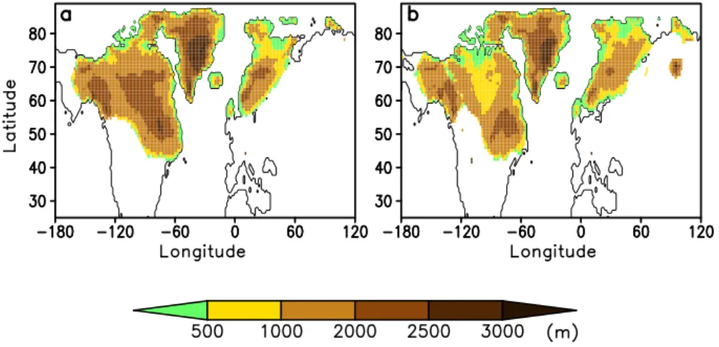
Fig. 8.Thickness of the simulated ice sheets when the maximum area of the entire simulation was achieved in experiment CC200(a)and REG200(b), respectively.
stability of the ice sheets by making them more sensitive to changes in orbital forcing. Only when a large area of North America is free of sediments, can the ice sheet survive sev-eral precessional cycles before it expands well into the area covered by the sediments, making the ice sheet more sensi-tive to summer insolation changes.
Glacial cycles simulated in the REG experiments have, for the same CO2 concentrations, considerably smaller
ampli-tude than in the CC experiments. Even for a CO2
concen-tration of 200 ppm, which is likely near the lower limit of CO2concentrations during the 40-kyr world (H¨onisch et al.,
2009), the maximum simulated NH ice volume for most of glacial cycles is within the range 30–40 m of sea level. This is significantly smaller then simulated by Bintanja and van de Wal (2008) but more in line with Siddall et al. (2010). Such a small magnitude of ice volume variations in the REG exper-iments has an important implication for the interpretation of benthicδ18O records, since it implies a much smaller relative contribution of the NH ice volume to the glacial-interglacial δ18O variations for the 40-kyr world compared to the 100-kyr world. At the same time, the maximum southward ex-tent of the Laurentide ice sheet in the REG200 experiment (Fig. 8) is similar to that simulated in the BE and CC200 experiments. This is consistent with paleoclimate evidence of a similar southward extent of the Laurentide ice sheet in the 40- and 100-kyr worlds reviewed by Clark et al. (2006). The large difference in volume for ice sheets with a similar area is explained by the fact that in the REG experiments, due to strong sliding over a broader sediment-covered area, the maximum thickness of the central part of the Laurentide ice sheet is much smaller than at the end of the long glacial cycles simulated in BE or CC200 experiments.
4 Discussion
The results presented above demonstrate that our model simulates long asymmetric glacial cycles both with realis-tic (time-dependent) and constant CO2concentrations for a
broad range of CO2 concentrations and model parameters.
The simulated long glacial cycles can be understood in the framework of the stability diagram of the climate-cryosphere system in the phase space of the orbital forcing (Calov and Ganopolski, 2005). According to this analysis, the inter-glacial state becomes unstable when summer insolation falls below a certain threshold value and the system enters the glacial state. Although the ice sheets experience both growth and decay during different phases of orbital forcing, the sys-tem remains in the domain of attraction of the glacial state most of time and, therefore, the ice volume has a general ten-dency to grow. Such a stability diagram, however, does not explain why glacial cycles are rapidly terminated ca. 100 kyr after their start. The explanation of glacial termination re-quires an additional strong nonlinear mechanism, which, in our case, is the dust feedback. This feedback is activated after the ice sheets spread well into the area covered by thick ter-restrial sediments. High rates of dust deposition over the ice sheets reduce their albedo, which enhances ablation and thus amplifies the ice sheet response to rising insolation. Note that this mechanism was already proposed by Peltier and Mar-shall (1995), but they treat this in a rather simplistic manner, namely, they prescribed two to three times higher ablation rates during termination only.
If large portions of the northern continents are cleared from terrestrial sediments, as is the case at present, the ice sheets can survive several insolation maxima before they spread into the area covered by the sediments and the mechanism described above is activated. This usually occurs after the minimum of eccentricity is reached, but the precise timing of glacial termination depends on the phase between obliq-uity and precession. For this reason, the timing of glacial terminations relative to the eccentricity minima can vary in a broad range (Huybers and Wunsch, 2005). However, even this rather general tendency of the NH ice sheets to grow during periods of low eccentricity and to terminate during the rise of eccentricity is sufficient to produce a sharp peak in the frequency spectrum of ice volume in the 100 kyr band. Although in our experiments the effects of fast ice sheet sliding and dust deposition are sufficient to terminate long glacial cycles, it is likely that other nonlinear processes also play an important role. Several such mechanisms have been proposed: accelerated flow and wastage at the southern tip of the ice sheet due to proglacial lakes and/or marine incursions (Pollard, 1983), large-scale instabilities of marine ice sheets (Peltier and Marshall, 1995). Another factor that contributes to the termination of glacial cycles is the rise of CO2during
glacial terminations (Wolff et al., 2009). However, the latter is rather a positive feedback in the Earth system than a cause of glacial termination.
Although the mechanisms of 100 kyr cyclicity presented here invoke the concept of phase locking, it is fundamentally different from the mechanism of phase locking ofinternal
oscillations in the climate-cryosphere or climate-cryosphere-carbonosphere system to the orbital forcing (e.g. Saltzman and Maasch, 1988; Paillard and Parrenin, 2004; Tziperman et al., 2006). In the latter case, glacial cycles with a typical periodicity of 100 kyr exist in the system even without orbital forcing (i.e. with constant orbital parameters). The orbital forcing only sets the precise timing of glacial terminations. In our case, glacial cycles are the response of the climate-cryosphere system to the orbital forcing and both 100 kyr cyclicity and the timing of terminations are set by the orbital forcing. If orbital parameters are fixed, our model does not simulate glacial cycles. More detailed comparison of these two concepts of glacial cycles will be given in forthcoming work.
5 Conclusions
Results of our experiments support the notion that 100 kyr cycles represent a direct, strongly nonlinear response of the climate-cryosphere system to orbital forcing and they are di-rectly related to the corresponding eccentricity period. In terms of nonlinear dynamics, this link can be interpreted as the phase-locking of the long glacial cycles to the shortest (100 kyr) eccentricity cycles. Physically, this phase-locking is explained by the fact that the ice sheets tend to grow
monotonously during periods of low eccentricity and reach their critical size (volume) around the minimum of eccen-tricity. When eccentricity starts to grow, the first sufficiently large positive anomaly in orbital forcing can lead to the rapid and irreversible meltback of the Northern Hemisphere ice sheets. This mechanism requires the existence of long glacial cycles that, in turn, require sufficiently low CO2
concentra-tions and a large area of the continents to be free of sedi-ment. The CO2concentration not only determines the
domi-nant regime of glacial variability, but also strongly amplifies 100 kyr cycles. Therefore, realistic simulations of the glacial cycles require comprehensive Earth system models that in-clude both physical and bio-geochemical components of the Earth system.
Acknowledgements. We would like to thank Ralf Greve for providing us with the ice sheet model SICOPOLIS and the two anonymous reviewers and Alexander Robinson for useful suggestions. This project was partly funded by the Deutsche Forschungsgemeinschaft CL 178/4-1 and CL 178/4-2.
Edited by: M. Siddall
References
Bauer, E. and Ganopolski, A.: Aeolian dust modeling over the past four glacial cycles with CLIMBER-2, Global Planet. Change, 74, 49–60, 2010.
Berger A.: Long-term variations of daily insolation and Quaternary climatic change, J. Atmos. Sci., 35, 2362–2367, 1978.
Berger, A., Loutre, M. F., and Gallee, H.: Sensitivity of the LLN climate model to the astronomical and CO2forcings over the last 200 ky, Clim. Dynam., 14, 615–629, 1998.
Berger, A., Li, X. S., and Loutre, M. F: Modeling northern hemi-sphere ice volume over the last 3 million years, Quaternary Sci. Rev., 18, 1–11, 1999.
Berger, A., Melice, J. L., and Loutre M. F.: On the origin of the 100-kyr cycles in the astronomical forcing, Paleoceanography, 20, PA4019, doi:10.1029/2005PA001173, 2005.
Bintanja, R. and van de Wal, R.: North American ice-sheet dynam-ics and the onset of 100,000-year glacial cycles, Nature, 454, 869–872, 2008.
Bonelli, S., Charbit, S., Kageyama, M., Woillez, M.-N., Ramstein, G., Dumas, C., and Quiquet, A.: Investigating the evolution of major Northern Hemisphere ice sheets during the last glacial-interglacial cycle, Clim. Past, 5, 329–345, doi:10.5194/cp-5-329-2009, 2009.
Brovkin, V., Bendtsen, J., Claussen, M., Ganopolski, A., Kubatzki, C., Petoukhov, V., and Andreev, A.: Carbon cycle, vegeta-tion and climate dynamics in the Holocene: experiments with the CLIMBER-2 model, Global Biogeochem. Cyc., 16, 1139, doi:10.1029/2001GB001662, 2002.
Calov, R., Ganopolski, A., Claussen, M., Petoukhov, V., and Greve. R.: Transient simulation of the last glacial inception, Part I: Glacial inception as a bifurcation of the climate system, Clim. Dynam., 24, 545–561, doi:10.1007/s00382-005-0007-6, 2005. Clark, P. U. and Pollard, D.: Origin of the Middle Pleistocene
Tran-sition by ice sheet erosion of regolith, Paleoceanography, 13, 1– 9, 1998.
Clark, P. U., Archer, D., Pollard, D., Blum, J. D., Rial, J. A., Brovkin, V., Mix, A. C., Pisias, N. G., and Roy, M.: The middle Pleistocene transition: characteristics, mechanisms, and implica-tions for long-term changes in atmosphericpCO2, Quaternary
Sci. Rev., 25, 3150–3184, 2006.
Claussen, M., Mysak, L. A., Weaver, A. J., Crucifix, M., Fichefet, T., Loutre, M. F., Weber, S. L., Alcamo, J., Alexeev, V. A., Berger, A., Calov, R., Ganopolski, A., Goosse, H., Lohman, G., Lunkeit, F., Mokhov, I. I., Petoukhov, V., Stone, P., and Wang, Z.: Earth system models of intermediate complexity: closing the gap in the spectrum of climate system models, Clim. Dynam., 18, 579–586, 2002.
Crowley, T. J. and Hyde, W. T.: Transient nature of late Pleistocene climate variability, Nature, 456, 226–230, 2008.
Deblonde, G. and Peltier, W. R.: Simulations of continental ice sheet growth over the last glacial-interglacial cycle: Experiments with a one-level seasonal energy balance model including realis-tic geography, J. Geophys. Res., 96, 9189–9215, 1991.
Duplessy, J.-C., Labeyrie, L., Juillet-Leclerc, A., Maitre, F., Duprat, J., and Sarnthein, M.: Surface salinity reconstruction of the North Atlantic Ocean during the last glacial maximum, Oceanol. Acta, 14, 311–324, 1991.
EPICA: Eight glacial cycles from an Antarctic ice core, Nature, 429, 623–628, 2004.
Ganopolski, A. and Roche, D.: On the nature of leads and lags dur-ing glacial-interglacial transitions, Quaternary Sci. Rev., 37/38, 3361–3378, 2009.
Ganopolski, A., Petoukhov, V., Rahmstorf, S., Brovkin, V., Claussen, M., Eliseev, A., and Kubatzki, C.: CLIMBER-2: a climate system model of intermediate complexity, Part II: Model sensitivity, Clim. Dynam., 17, 735–751, 2001.
Ganopolski, A., Calov, R., and Claussen, M.: Simulation of the last glacial cycle with a coupled climate ice-sheet model of interme-diate complexity, Clim. Past, 6, 229–244, doi:10.5194/cp-6-229-2010, 2010.
Gildor, H. and Tziperman, E.: A sea ice climate switch mechanism for the 100-kyr glacial cycles, J. Geophys. Res., 106, 9117–9133, 2001.
Greve, R.: A continuum-mechanical formulation for shallow poly-thermal ice sheets, Philos. T. Roy. Soc. Lond. A, 355, 921–974, 1997.
Hays, J. D., Imbrie, J., and Shackleton, N. J.: Variations in the earth’s orbit: pacemaker of the Ice Ages, Science, 194, 1121– 1132, 1976.
Herbert, T. D., Peterson, L. C., Lawrence, K. T., and Liu, Z.: Trop-ical Ocean Temperatures Over the Past 3.5 Million Years, Sci-ence, 328, 1530–1534, 2010.
H¨onisch, B., Hemming, N. G., Archer, D., Siddall, M., and Mc-Manus, J. F.: Atmospheric carbon dioxide concentration across the Mid-Pleistocene transition, Science, 324, 1551–1554, 2009.
Holden, P. B., Edwards, N. R., Wolff, E. W., Lang, N. J., Singarayer, J. S., Valdes, P. J., and Stocker, T. F.: Interhemispheric coupling, the West Antarctic Ice Sheet and warm Antarctic interglacials, Clim. Past, 6, 431–443, doi:10.5194/cp-6-431-2010, 2010. Huybers, P. and Wunsch, C.: Obliquity pacing of the late
Pleis-tocene glacial terminations, Nature, 434, 491–494, 2005. Huybrechts, P.: Sea-level changes at the LGM from ice-dynamics
reconstructions of the Greenland and Antarctic ice sheets during the glacial cycles, Quaternary Sci. Rev., 21, 203–231, 2002. Imbrie, J., Berger, A., Boyle, E. A., Clemens, S. C., Duffy, A.,
Howard, W. A., Kukla, G., Kutzbach, J., Martinson, D. G., McIn-tyre, A., Mix, A. C., Molfino, B., Morley, J. J., Peterson, L. C., Pisias, N. G., Prell, W. G., Raymo, M. E., Shackleton, N. J., and Toggweiler, J. R.: On the structure and origin of major glaciation cycles, 2. The 100,000-year cycle, Paleoceanography, 8, 699– 735, 1993.
Jouzel, J., Masson-Delmotte, V., Cattani, O., Dreyfus, G., Falourd, S., Hoffmann, G., Minster, B., Nouet, J., Barnola, J. M., Chap-pellaz, J., Fischer, H., Gallet, J. C., Johnsen, S., Leuenberger, M., Loulergue, L., Luethi, D., Oerter, H., Parrenin, F., Raisbeck, G., Raynaud, D., Schilt, A., Schwander, J., Selmo, E., Souchez, R., Spahni, R., Stauffer, B., Steffensen, J. P., Stenni, B., Stocker, T. F., Tison, J. L., Werner, M., and Wolff, E. W.: Climate variability over the past 800 000 years, Science, 317, 793–796, 2007. Lisiecki, L. E.: Links between eccentricity forcing and the
100,000-year glacial cycle, Nat. Geosci., 3, 349–352, 2010.
Lisiecki, L. E. and Raymo, M. E.: A Pliocene-Pleistocene stack of 57 globally distributed benthicδ18O records, Paleoceanography, 20, PA1003, doi:10.1029/2004PA001071, 2005.
Mahowald, N., Muhs, D. R., Levis, S., Rasch, P. J., Yoshioka, M., Zender, C. S., and Luo, C.: Change in atmospheric mineral aerosols in response to climate: Last glacial period, preindustrial, modern, and doubled carbon dioxide climates, J. Geophys. Res., 111, D10202, doi:10.1029/2005JD006653, 2006.
Milankovitch, M.: Kanon der Erdbestrahlung und Seine Andwen-dung auf das Eiszeitenproblem, Royal Serbian Academy Special Publication, 132, Belgrade, Serbia, 1941.
NGRIP: High-resolution record of Northern Hemisphere climate extending into the last interglacial period, Nature, 431, 147–151, 2004.
Paillard, D.: The timing of Pleistocene glaciations from a simple multiple-state climate model, Nature, 391, 378–381, 1998. Paillard, D.: Glacial cycles: Toward a new paradigm, Rev.
Geo-phys., 39, 325–346, 2001.
Paillard, D. and Parrenin, F.: The Antarctic ice sheet and the trig-gering of deglaciations, Earth Planet. Sc. Lett., 227, 263–271, 2004.
Peltier, W. R. and Marshall, S.: Coupled energy-balance/ice sheet simulations of the glacial cycle: A possible connection between terminations and terrigenous dust, J. Geophys. Res., 100, 14269– 14289, 1995.
Petoukhov, V., Ganopolski, A., Brovkin, V., Claussen, M., Eliseev, A., Kubatzki, C., and Rahmstorf, S.: CLIMBER-2: A climate system model of intermediate complexity, Part I: Model descrip-tion and performance for present climate, Clim. Dynam., 16, 1– 17, 2000.
Pollard, D.: A coupled climate-ice sheet model applied to the Qua-ternary ice ages, J Geophys. Res., 88, 7705–7718, 1983. Ridgwell, A. J., Watson, A. J., and Raymo, M. E.: Is the
spec-tral signature of the 100 kyr glacial cycle consistent with a Mi-lankovitch origin?, Paleoceanography, 14, 437–440, 1999. Ruddiman, W. F., Raymo, M. E., Martinson, D. G., Clement, B. M.,
and Backman, J.: Pleistocene evolution: Northern hemisphere ice sheets and North Atlantic Ocean, Paleoceanography, 4, 353– 412, 1989.
Saltzman, B. and Maasch, K.A.: Carbon cycle instability as a cause of the late Pleistocene ice age oscillations: Modeling the asym-metric response, Global Biogeochem. Cy., 2, 177–185, 1988. Siddall, M., H¨onisch, B., Waelbroeck, C., and Huybers, P.: Changes
in deep Pacific temperature during the mid-Pleistocene transition and Quaternary, Quaternary Sci. Rev., 29, 170–181, 2010. Svendsen, J., Alexanderson, H., Astakhov, V., Demidov, I.,
Dowdeswell, J., Funder, S., Gataullin, V., Henriksen, M., Hjort, C., Houmark-Nielsen, M., Hubberten, H., Ingolfsson, O., Ja-cobsson, M., Kjaer, K., Larsen, E., Lokrantz, H., Lunkka, J., Lysa, A., Mangerud, J., Matioushkov, A., Murray, A., M¨oller, P., Niessen, F., Nikolskaya, O., Polyak, L., Saarnisto, M., Siegert, C., Siegert, M., Spielhagen, R., and Stein, R.: Late Quaternary ice sheet history of northern Eurasia, Quaternary Sci. Rev., 23, 1229–1271, 2004.
Tziperman, E., Raymo, E., Huybers, P., and Wunsch, C.: Conse-quences of pacing the Pleistocene 100 kyr ice ages by nonlinear phase locking to Milankovitch forcing, Paleoceanography, 21, PA4206, doi:10.1029/2005PA001241, 2006.
Waelbroeck, C., Labeyrie, L., Michel, E., Duplessy, J. C., Mc-Manus, J. F., Lambeck, K., Balbon, E., and Labracherie, M.: Sea-level and deep water temperature changes derived from ben-thonic foraminifera isotopic records, Quaternary Sci. Rev., 21, 295–305, 2002.
Wolff, E. W., Fischer, H., and Rothlisberger, R.: Glacial termi-nations as southern warmings without northern control, Nat. Geosci., 2, 206–209, 2009.