HISTORICAL GIS DATA AND CHANGES IN URBAN MORPHOLOGICAL
PARAMETERS FOR THE ANALYSIS OF URBAN HEAT ISLANDS IN HONG KONG
F. Peng a, M.S. Wong a,*, J.E. Nichol a, P.W. Chanb
a Department of Land Surveying and Geo-Informatics, The Hong Kong Polytechnic University, Hong Kong – [email protected]; [email protected]; [email protected]
b Hong Kong Observatory, Hong Kong - [email protected]
Commission II, WG II /1
KEY WORDS: 3D building model, aerial photogrammetry, digital surface model, land surface temperature, urban morphological parameter
ABSTRACT:
Rapid urban development between the 1960 and 2010 decades have changed the urban landscape and pattern in the Kowloon Peninsula of Hong Kong. This paper aims to study the changes of urban morphological parameters between the 1985 and 2010 and explore their influences on the urban heat island (UHI) effect. This study applied a mono-window algorithm to retrieve the land surface temperature (LST) using Landsat Thematic Mapper (TM) images from 1987 to 2009. In order to estimate the effects of local urban morphological parameters to LST, the global surface temperature anomaly was analysed. Historical 3D building model was developed based on aerial photogrammetry technique using aerial photographs from 1964 to 2010, in which the urban digital surface models (DSMs) including elevations of infrastructures and buildings have been generated. Then, urban morphological parameters (i.e. frontal area index (FAI), sky view factor (SVF)), vegetation fractional cover (VFC), global solar radiation (GSR), Normalized Difference Built-Up Index (NDBI), wind speed were derived. Finally, a linear regression method in Waikato Environment for Knowledge Analysis (WEKA) was used to build prediction model for revealing LST spatial patterns. Results show that the final apparent surface temperature have uncertainties less than 1 degree Celsius. The comparison between the simulated and actual spatial pattern of LST in 2009 showed that the correlation coefficient is 0.65, mean absolute error (MAE) is 1.24 degree Celsius, and root mean square error (RMSE) is 1.51 degree Celsius of 22,429 pixels.
1. INTRODUCTION
The surface temperature is one of the main urban climatic parameters (Voogt and Oke, 2003). Some studies have investigated the effect of urbanization to regional warming (Christy and Goodridge, 1995; Dai et al., 1999; Diem et al., 2005; Lam, 2006; Lau and Ng, 2013). Hong Kong has the highest population density district in the world (Zhang, 2000). Understanding how the urban climatic changes caused by the past urban landscapes can permit planners and authorities to have the perspective for urban planning and design.
Human activities changes the natural environment, which lead to the reductions of natural surface and long-wave emission of surface, release of atmosphere pollutants and waste heats. These artificial factors determine the urban climate (Oke, 1978; Landsberg, 1987; Goldreich, 1995; Gomez et al., 1998). Thermal remote sensing of urban surface temperatures observes land surface temperature (LST) effectively in related to the surface energy balance.
Taha (1997) found the variations of surface albedo and vegetation cover are the controlling factors of climate. It has been proved that a negative correlation existed between Normalized Difference Vegetation Index (NDVI) and temperature (Chen et al. 2006, Zhang and Wang 2008), but a positive correlation is shown between Normalized Difference Build-up Index (NDBI) and temperature (Chen et al. 2006). Higher wind speed reduces the temperature differences inside the canopy layer due to inner atmospheric turbulent mixing and advection activity (Oke, 1982). Kolokotroni et al. (2006)
investigated the upper limit of heat island intensity, which increased until a certain wind speed and then gradually declined as the wind speed increased.
Currently, most researchers have focused on studying the spatial and temporal distribution, cause and effect, as well as the prediction model of the urban climate. This study aims to investigate the relationship between the urban morphology of a high density city and its urban climatic characteristics from a historical perspective. And, it will help predict the spatial distribution of urban surface temperature in the future based on the predictable morphologic factors. Our research team has developed historical 3D building morphological models between the 1964 and 2010. Following urban morphological parameters (i.e. FAI, SVF), VFC, NDBI, and GSR were calculated between the 1985 and 2010, LST data between the 1987 and 2009 were retrieved from historical Landsat images data. Finally, a linear regression method in WEKA was used to predict spatial patterns of LST.
2. STUDY AREA AND DATA USED
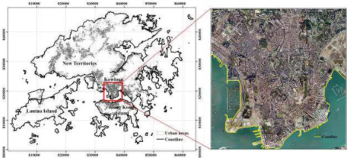
The Kowloon Peninsula in Hong Kong (Figure 1), a highly urbanized with an area of 160 km2 and an average population density of 44,917 persons/km2 in 2011 (Population Census, 2011), is selected as the study area. The Mongkok district in the Kowloon Peninsula has the largest population density in the world (130,000 persons/km2) (Boland, 2013). Kowloon has one large park (Kowloon Park) and a few small diverse urban parks, which separate built-up landscape in general. The topography is mainly flat, but goes up to 300 m in the northern of the The International Archives of the Photogrammetry, Remote Sensing and Spatial Information Sciences, Volume XLI-B2, 2016
Peninsula. Since the core areas in Kowloon is over 3 km from the coast, it has been strongly believed that the “wall effect” prevents cool sea breezes from penetrating to the inner city.
Figure 1. The study area: Kowloon Peninsula in Hong Kong (The right: DOM in 2014)
Hong Kong is under humid sub-tropical climate. Daily mean air temperatures range generally between 16.1 °C to 28.7 °C, but some abnormal temperatures also occur, e.g. the lowest temperatures ever recorded by the Hong Kong Observatory (HKO) are 0.0 °C on 18 January 1893 (HKO, 2003).
Table 1 shows that thermal infrared images acquired by Landsat 4 and 5 TM and Landsat 7 ETM+ sensors from 1987 onwards were used to derive LST data, as well as images from Landsat 2, 3, 4, 5 and 7 TM from 1975 onwards were used to calculate NDVI. In the previous study, buildings heights and buildings footprints data between the 1964 and 2010 were obtained from aerial photographs.
Date (yyyy/mm/dd) Time (GMT)
Spacecraft Cloud cover
1975/12/24 02:10 Landsat 2 0% 1979/10/19 02:10 Landsat 3 0% 1987/12/08 02:20 Landsat 5 0% 1990/12/24 02:17 Landsat 4 10% 1995/12/30 01:54 Landsat 5 0% 2000/11/01 02:42 Landsat 7 0% 2005/11/23 02:40 Landsat 5 12% 2009/12/04 02:42 Landsat 5 6%
Table 1. Landsat images data between the 1975 and 2009 in Hong Kong
3. LST RETRIEVAL
In the study, the LST data were converted from the raw digital numbers (DN) in thermal infrared band 6 using the mono-window algorithm. The calibration parameters on the satellite sensor and the Planck equation developed were used to calculate the brightness temperature. The parameters include upwelling and downwelling atmospheric radiances, atmospheric transmittance and surface emissivity. After atmospheric correction and emissivity calculation, surface temperature was calculated from brightness temperature. Specifically, LST at 30 m spatial resolution from Landsat image data was retrieved through the following four steps:
(1) Conversion from digital number to radiance
The DN were transformed into radiances using the TM post-calibration dynamic ranges provided by Markham and Barker (1986), which is described as:
LGainDNBias (1)
where L is the spectral radiance at the sensor's aperture, the
Gain and Biasare band-specific rescaling factors, which are
obtained from the metafile of the image.
(2) Land surface emissivity estimation
The thermal infrared band emissivity were simulated as a weighted mean according to tabulated numbers published by Masuda et al. (1988) using:
max min
max min
, ,
b
x y f d L x y
f d
(2)where
is the narrowband emissivity based on land use type, such as impervious surface area, vegetation, buildings areas. f
is the spectral response function (Markham and Barker, 1985).(3) Atmospheric correction
The Top of Atmospheric (TOA) radiances were then converted to surface-leaving radiance by removing the effects of the atmosphere in the thermal region. Specifically, the radiosonde launched near the study area at 0:00 GMT including geopotential, pressure, temperature, relative humidity and ozone profiles allow us to estimate the atmospheric transmissivity and atmospheric upwelling and downwelling radiances by MODTRAN 4.0 (Abreu and Anderson, 1996). The atmospheric profiles data with 27 pressure levels are provided by European centre for Medium-Range Weather Forecasts (ECMWF). Atmospheric data are available globally every 6 h and every 0.125 degree in latitude and longitude. Then, surface-leaving radiance will be calculated using the following equation (Barsi et al., 2005).
1
T
L L L L (3)
where LT is the blackbody radiance of kinetic temperature T,
L is the space-reaching or top-of-atmospheric radiance
measured by the instrument, L is the upwelling atmospheric radiance,
is the total atmospheric transmissivity between the surface and the sensor, L is the downwelling atmospheric radiance, L and L were calculated using a radiative transfer code e.g. MODTRAN (Berk et al., 1989), is the land surface emissivity.Date (yyyy/mm/dd)
Transmittance Upwelling radiance
Downwelling radiance
1987/12/08 0.82 1.19 1.95
1990/12/24 0.81 1.38 2.25
1995/12/30 0.95 0.32 0.59
2000/11/01 0.65 2.49 3.71
2005/11/23 0.72 2.05 3.16
2009/12/04 0.76 1.64 2.60
Table 2. Atmospheric correction parameter
(4) Surface temperature
Lastly, the radiances calculated were converted to surface temperature using the Landsat specific estimate of the Planck curve (Chander and Markham, 2003):
2 ln 1 1 273.15
B
T K K L (4)
where TB is the temperature in degree Celsius (°C),
K
1 and2
K
are pre-launch calibration constants. For Landsat 5 TM,1
K =607.76 Wm-2sr-1μm-1 and
2
K =1260.56 K; For Landsat 4
TM, K1=671.62 Wm
-2sr-1μm-1 and
2
K =1284.30 K; For Landsat
7 TM, K1=666.09 Wm
-2sr-1μm-1 and
2
K =1282.71 K; L is the
spectral radiance.
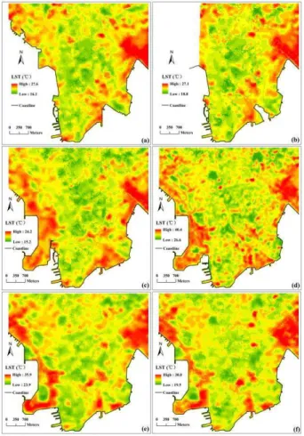
To validate the atmospheric correction, sea surface temperature (SST) was calculated with emissivity of 1.0 in the years of 2005 and 2009. SST retrieved and observed at the Waglan Island station are 23.7 °C and 23.1 °C in 2005, 19.1 °C and 19.9 °C in 2009. The apparent surface temperatures have uncertainties less than 1 °C when the atmosphere is relatively clear. Figure 2 shows the spatial distribution of the retrieved LST between the 1987 and 2009, and densely high rise areas appear cool on daytime images, which is consistent with the previous study in Hong Kong (Nichol, 2005).
Figure 2. Spatial pattern of LST in the Kowloon Peninsula at 30 m spatial resolution (a): 1987; (b): 1990; (c): 1995; (d): 2000;
(e): 2005; (f): 2009
Many researches have suggested that increasing greenhouse gases may result in global warming. The effect of climate change on urban environment should be considered as
composed by global and local urban climate change. From the Royal Netherlands Meteorological Institute (KNMI) climate explorer (http://www.climexp.knmi.nl), global mean temperature of Coupled Model Intercomparison Project Phase (CMIP5) monthly historical and Representative Concentration Pathways (RCPs) are derived from mean value of multi-model (e.g. ACCESS1-0, BNU-ESM, CCSM4, CESM1-CAM5, CMCC-CM, CNRM-CM5), and give the temperature anomaly relative to the mean temperature of the 1951–1980 reference period. These data depict how much global region have been warmed or cooled compared with a base period of 1951-1980. The RCP database aims at documenting the emissions, concentrations, and land-cover change projections. In the study, the global mean temperature chosen is modelled using RCP 6.0, which is developed by the Asia-Pacific Integrated Model (AIM) modelling team at the National Institute for Environmental Studies (NIES) in Japan (Fujino et al., 2006; Hijioka et al., 2008). Table 3 shows global temperature anomaly between the 1987 and 2009 which can help to reduce the effect of global warming in the study area.
Date (yyyy/mm/dd) Mean LST (°C) Global temperature anomaly (°C)
1987/12/08 21.8 0.29
1990/12/24 22.8 0.41
1995/12/30 19.3 0.32
2000/11/01 30.9 0.61
2005/11/23 29.3 0.76
2009/12/04 23.4 0.75
Table 3. The mean LST and global temperature anomaly
4. POTENTIAL IMPACT FACTORS
4.1 VFC, NDBI
The VFC and NDBI indices were used to characterize the land use and land cover (LULC) types and used to evaluate the quantitative relationships between LULC types and LST. NDVI was calculated using the following equation.
4 3
4 3
b b NDVI
b b
(5)
where b3 is the reflectance value of red band (band 3) and b4 is
the reflectance value of near-infrared band (band 4) from the Landsat images. The NDVI values range from −1 to 1, and positive values indicating vegetated areas, negative values signifying non-vegetated surface features. Gutman and Ignatov (1998) used a dense vegetation mosaic-pixel model to derive the VFC by scaled NDVI, which is defined as,
min
max min
NDVI NDVI f
NDVI NDVI
(6)
where NDVImin and NDVImax correspond to the values of NDVI
for bare soil and a surface with a VFC of 100%, respectively. In theory, NDVImin should be zero for most soil types, but changes
from -0.1 to 0.2 (Carlson and Ripley, 1997; Rundquist, 2002), due to the influences of many factors. NDVImax should be the
max of NDVI, but subject to the spatial or temporal change, due to the influences of vegetation type. Thus, NDVImax and
min
NDVI are not fixed value (Kaufman and tanre, 1992; Qi et al.,
1994), even in the same image. According to the size of VFC, the medium-high (0.5< VFC ≤ 0.7) and high (0.7 < VFC) vegetation cover were chosen as vegetation areas in the study.
NDBI (Equation (7)) as an index is sensitive to the built-up area (Zha et al., 2003).
5 4
5 4
b b NDBI
b b
(7)
where b5 and b4 are the respective DN of mid-infrared band
(band 5) and near-infrared band (band 4) of the Landsat images.
4.2 SVF calculating using a raster DSM
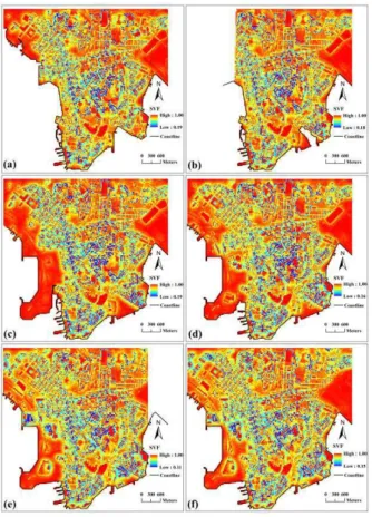
The SVF is defined by the ratio between radiation received from a flat surface and the entire hemispheric radiation environment (Watson and Johnson 1987). The range of the SVF is between 0 and 1, and closes to 1 in perfectly flat terrain, and decreases proportionally in these locations with obstructions such as buildings and trees, reaches to 0 in a completely obstructed location means that all outgoing radiation and received diffuse solar radiation will be intercepted by obstacles (Oke 1993; Brown and Grimmond 2001).
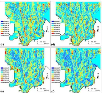
The software of calculating the SVF can be downloaded from (IAPS ZRC SAZU, 2010), which is implemented using the remote sensing software ENVI+IDL (ITT Visual Information Solutions, 2010). In SVF calculation, the DSM data were resampled to 30 meter resolution for maintaining the consistent spatial scale with LST data and input into the software, searching radius is 90 m (3 pixels) in 16 directions. Figure 3 shows the spatial distribution of SVF values in the study area.
Figure 3. Spatial distribution of SVF at 30 spatial resolution. (a): 1985; (b): 1990; (c): 1995; (d): 2000; (e): 2005; (f): 2010
4.3 FAI derived from a GIS-based method
For urban renewal study, it is essential to facilitate a measure to estimate wind condition in respects to the geometry and orientation of buildings.
In the study, the frontal area (FA) was calculated by inputting raster data with the height information, wind direction, and backward flow coefficient in a GIS-based program. From the perspective of scale assimilation, buildings vector data was first converted to raster data at 30 m spatial resolution. Figure 4 demonstrates the prototype of FAI calculation developed in ArcGIS Engine and Visual C# program environment based on .NET Framework platform.
Figure 4. The parameter setting window of the FAI calculation
The FAI is the total area of building facets projected to plane normal facing the particular wind direction. The FAI is the FA divided by the plane area (Burian et al., 2002; Grimmond and Oke, 1999; Wong et al., 2010) (Equation (8))
_
FAIFA Area grid (8)
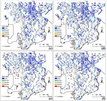
Where FAI is the frontal area index, FA is the frontal area, Area_grid is the grid area (900 m2 in the study). Figure 5 shows the FAI values of the Kowloon Peninsula in east-west direction at 30 m spatial resolution from 1985 to 2010, in which nodata indicates that wind flow of the ground objects was blocked and sea surface did not take part in FA calculation. Due to east wind of high frequency in Hong Kong, FAI values were calculated easterly wind movement towards the west.
Figure 5. Spatial distribution of FAI at 30 spatial resolution. (a): 1985; (b): 1990; (c): 1995; (d): 2000; (e): 2005; (f): 2010
4.4 Simulation of GSR
The GSR received by topography and surface features is a function including the geometry of the earth, atmospheric transmittance, geographical location, sun elevation angle, orientation (slope and aspect), and elevation (Allen et al., 2006). The solar radiation derives from the sun, which will be intercepted as direct, diffuse, and reflected components, the three radiation forms the GSR. The solar radiation analysis tool in the ArcGIS Spatial Analyst extension maps and analyses the global solar radiation over a geographic area at specific time periods (ESRI Inc., 2015). The GSR does not include reflected radiation, as the direct radiation is the principal component, secondly is the diffuse radiation. The DSM data were resampled to 30 meter resolution and input into ArcGIS software for calculating GSR at a specific time period. The fraction of radiation passing through the atmosphere as an important factor is calculated by the average of transmissivity values of all wavelengths. And, the average values of transmissivity from all wavelengths were estimated by the MODTRAN 4.0. Figure 6 shows that GSR including direct radiation and diffuse radiation which was modelled based on the transmissivity values in Table 4. Then, the simulated GSR values in the King’s park extracted, according to the geographical location, were used for evaluating the accuracy. Table 4 shows that the maximum difference and minimum difference between observed GSR and simulated GSR at King’s park station from 1987s onwards is 0.09 MJ/m2 and 0.00 MJ/m2, respectively.
Date
(yyyy/mm/dd) Transmissivity
GSR (unit:MJ/m2) Error Model
value
King’s park
1987/12/08 0.59 2.15 2.14 0.01
1990/12/24 0.58 1.90 1.90 0.00
1995/12/30 0.66 2.04 2.05 -0.01
2000/11/01 0.56 2.23 2.32 -0.09
2005/11/23 0.57 2.03 2.07 -0.04
2009/12/04 0.58 1.93 1.96 -0.03
Table 4. A comparison between observed and simulated GSR
Figure 6. Spatial distribution of GSR at a specific time from 1987 to 2009. (a): 1987; (b): 1990; (c): 1995; (d): 2000; (e):
2005; (f): 2009
4.5 Simulation of Air flow
An ArcGIS extension named Airflow Analysis was used to calculate the wind speed in the study. The model has been developed by Kyushu University. It provides complex calculations, mesh generation, wind simulation, and 2D/3D visualization integrated into ArcGIS version 10.3, and the results can be used for further spatial analysis in ArcGIS. The wind speed was calculated by inputting building footprints and height attributes into the Airflow Analysis tool. Figure 7 shows the normalized values of average wind speed in east-west direction using Airflow Analysis module.
Figure 7. Spatial distribution of the normalized value of wind speed in east-west direction from 1985 to 2010. (a): 1985; (b):
1990; (c): 1995; (d): 2000; (e): 2005; (f): 2010
5. PREDICTION MODEL
The WEKA is a significant and systemic workbench in data mining and machine learning. It not only provides a toolbox about learning algorithms, but also a framework in which new algorithms can be implemented without the support of infrastructure data manipulation and program evaluation (Hall et al., 2009).
The WEKA software package was downloaded from Machine Learning Group (2013). Classifiers as main learning methods in WEKA include a series of rule sets and decision trees for data modelling. Moreover, the command interface in WEKA also includes visualization tools and algorithms for data analysis and predictive modelling (Frank et al., 2004). In the study, VFC, NDBI, FAI, GSR, building height, SVF, wind speed, altitude, longitude, and time after multicollinearity analysis were selected as attributes to predict the spatial distribution of LST. The correlation coefficient was used to measure the accuracy on the predictions. And the correlation coefficients from the method of linear regression, Reduced Error Pruning Tree (REPTree) (a fast decision tree learner), instance-based learners (IBk) (k-nearest neighbour learner), model trees and rules (M5Rules) are 0.65, 0.59, 0.33, and 0.61, respectively. As a result, it is found that linear regression will be the best in predicting the spatial pattern of LST. Figure 8 shows the predicted spatial pattern of LST in 2009, which was used to compare with the spatial distribution of LST retrieved from Landsat image. It can be found that the differences of maximum LST and minimum LST are 2 °C, 1 °C, respectively. Furthermore, it can also be found by analysis of pixel-to-pixel that the correlation coefficient is 0.65, MAE is 1.24 degree Celsius, and RMSE is 1.51 degree Celsius of 22,429 pixels.
Figure 8. Comparison between simulated and actual spatial pattern of LST in 2009
6. CONCLUSION
In the study, spatial and temporal characteristics were analyzed about the relationships between factors (VFC, NDBI, SVF, FAI, building height, GSR, wind speed) and LST. And, these factors are demonstrated the usefulness for the prediction of LST. Ultimately, it is found that a linear regression method outperformed in predicting the spatial pattern of LST, which can be verified by the comparison between the simulated and actual spatial pattern of LST in 2009.
ACKNOWLEDGEMENTS
This work was supported in part by the grant of Early Career Scheme (project id: 25201614), the grant HKU9/CRF/12G of Collaborative Research Fund from the Research Grants Council of Hong Kong; the grant G-YM85 from the Hong Kong Polytechnic University. The authors thanks the Hong Kong Civil Engineering and Development Department for the airborne Lidar data, the Hong Kong Lands Department for building GIS data, the Hong Kong Observatory for the weather and climate data, and NASA LP DAAC for the Landsat satellite imagery.
REFERENCES
Abreu, L. W., Anderson, G. P., 1996. The MODTRAN 2/3 report and LOWTRAN 7 model. Contract, 19628(91-C): 0132.
Allen, R. G., Trezza, R., Tasumi, M., 2006. Analytical integrated functions for daily solar radiation on slopes. Agricultural and Forest Meteorology, 139(1), pp. 55-73.
Barsi, J. A., Schott, J. R., Palluconi, F. D., Hook, S. J., 2005. Validation of a web-based atmospheric correction tool for single thermal band instruments. In Optics & Photonics 2005, International Society for Optics and Photonics.
Berk, A., Bernstein, L. S., Robertson, D. C., 1989. MODTRAN: A Moderate Resolution Model for LOWTRAN 7, Technical Report GL-TR-89-0122, Geophys. Lab, Bedford, MA.
Boland, R. Mongkok Ladies Market Tour. http://gohongkong.about.com/od/whattoseeinhk/ss/MongkokLa diesMa.htm (6 Apr. 2013).
Brown, M. J., Grimmond, C. S. B., 2001. Sky view factor measurements in downtown Salt Lake City: data report for the DOE CBNP URBAN Experiment October 2000. Internal Report Los Alamos National Laboratory, Los Alamos, New Mexico, LA-UR-01–1424.
Burian, S. J., Brown, M. J., Linger, S. P., 2002. Morphological analysis using 3D building databases (pp. 36–42). Los Angeles, CA: Los Alamos National Laboratory. [LA-UR-02-0781].
Carlson, T. N., Ripley, D. A., 1997. On the relation between NDVI, fractional vegetation cover, and leaf area index. Remote Sensing of Environment, 62(3), pp. 241–252.
Chander, G., Markham, B., 2003. Revised Landsat-5 TM radiometric calibration procedures and postcalibration dynamic ranges. IEEE Transactions on Geoscience and Remote Sensing, 41(11), pp. 2674-2677.
Chen, X. L., Zhao, H. M., Li, P. X., Yin, Z.Y., 2006. Remote sensing image-based analysis of the relationship between urban heat island and land use/cover changes. Remote sensing of environment, 104(2), pp. 133-146.
Christy, J.R., Goodridge, J., 1995. Precision global temperatures from satellites and urban warming effects of non-satellite data. Atmospheric Environment, 29 (16), pp. 1957– 1961.
Dai, A., Trenberth, K. E., Karl, T. R., 1999. Effects of clouds, soil moisture and water vapor on diurnal temperature range. Journal of Climate, 12(8), pp. 2451–2473.
Diem, J. E., Ricketts, C. E., Dean, J. R., 2006. Impacts of urbanization on land-atmosphere carbon exchange within a metropolitan area in the USA. Climate Research, 30(3), pp. 201–213.
ESRI Inc. 2015. ArcGIS spatial analyst for area solar radiation. ESRI ArcGIS 10.1. http://resources.arcgis.com/ en/help/main/10.1/index.html#/Area_Solar_Radiation/009z000 000t5000000/ (29 Dec. 2015).
Frank, E., Hall, M., Trigg, L., Holmes, G., Witten, I. H., 2004. Data mining in bioinformatics using Weka. Bioinformatics, 20(15), pp. 2479-2481.
Fujino, J., Nair, R., Kainuma, M., Masui, T., Matsuoka, Y., 2006. Multi-gas mitigation analysis on stabilization scenarios using AIM global model. The Energy Journal, 3, pp. 343-353.
Goldreich, Y., 1995. Urban climate studies in Israel—a review. Atmospheric Environment, 29 (4), pp. 467–478.
Gomez, F., Gaja, E., Reig, A., 1998. Vegetation and climatic changes in a city. Ecological Engineering, 10 (4), pp. 355–360. Gutman, G., Ignatov, A., 1998. The derivation of the green vegetation fraction from NOAA/AVHRR data for use in numerical weather prediction models. International Journal of remote sensing, 19(8), pp. 1533-1543.
Grimmond, C. S. B., Oke, T. R., 1999. Aerodynamic properties of urban areas derived from analysis of surface form. Journal of Appllied Meteorology, 38, pp. 1262–1292.
Hall, M., Frank, E., Holmes, G., Pfahringer, B., Reutemann, P., Witten, I. H., 2009. The WEKA data mining software: an update. ACM SIGKDD explorations newsletter, 11(1), pp. 10-18.
Hijioka, Y., Matsuoka, Y., Nishimoto, H., Masui, M. Kainuma, M., 2008. Global GHG emissions scenarios under GHG
concentration stabilization targets. Journal of Global Environmental Engineering, 13, pp. 97-108.
Hong Kong Observatory: Hong Kong Observatory. Hong Kong; 2003.
IAPS ZRC SAZU. 2010. Institute of Anthropological and Spatial Studies ZRC SAZU. Sky-View Factor. Available online: http://iaps.zrc-sazu.si/index.php?q=en//node/138 (20 Dec. 2013).
ITT Visual Information Solutions. 2010. ENVI Software: Image processing & analysis solutions. 2010; Available online: http://www.ittvis.com/ProductServices/ENVI.aspx (9 Nov. 2013).
Kaufman, Y., Tanre, D., 1992. Atmospherically resistant vegetation index (ARVI) for EOS-MODIS. IEEE Transactions on Geoscience and Remote Sensing 30, pp. 261–270.
Kolokotroni, M., Giannitsaris, I., Watkins, R., 2006. The effect of the London urban heat island on building summer cooling demand and night ventilation strategies. Solar Energy, 80(4), pp. 383-392.
Lam, K. S., Chan, D. W. T., Chan, E. H. W., Tai, C. T., Fung, W. Y., Law, K. C., 2006. Infiltration of outdoor air in two newly constructed high rise residential buildings. International journal of ventilation, 5(2), pp. 249-258.
Lau, K. L., Ng, E., 2013. An investigation of urbanization effect on urban and rural Hong Kong using a 40-year extended temperature record. Landscape and Urban Planning, 114, pp. 42-52.
Machine Learning Group. 2013. Machine Learning Group at the University of Waikato. Weka. Available online: http://www.cs.waikato.ac.nz/~ml/weka/index.html. (12 Oct. 2014).
Markham, B. L., Barker, J. L., 1985. Spectral characterization of the Landsat Thematic Mapper sensors. International Journal of Remote Sensing, 6(5), pp. 697-716.
Markham, B. L., Barker, J. L., 1986. Landsat MSS and TM post-calibration dynamic ranges, exoatmospheric reflectances and at-satellite temperatures. EOSAT Landsat technical notes, 1(1), pp. 3-8.
Masuda, K., Takashima, T., Takayama, Y., 1988. Emissivity of pure and sea waters for the model sea surface in the infrared window regions. Remote Sensing of Environment, 24(2), pp. 313-329.
Nichol, J. 2005. Remote sensing of urban heat islands by day and night. Photogrammetric Engineering & Remote Sensing, 71(5), pp. 613-621.
Oke T.R., 1978. Boundary layer climates. London: Methuen.
Oke, T. R., 1982. The energetic basis of the urban heat island. Quarterly Journal of the Royal Meteorological Society, 108, pp. 1-24.
Oke, T.R., 1993. Boundary Layer Climates. 2nd edition. Cambridge: Cambridge University Press.
Population Census – Summary Results. 2011 Population Census Office Census and Statistics Department.
Qi, J., Kerr, Y., Chehbouni, A., 1994. External factor consideration in vegetation index development. Proceedings of 6th International Symposium on Physical Measurements and Signatures in Remote Sensing, France, pp. 723–730.
Rundquist, B.C., 2002. The influence of canopy green vegetation fraction on spectral measurements over native tall grass prairie. Remote Sensing of Environment, 81(1), pp. 129– 135.
Taha, H., 1997. Urban climates and heat islands: albedo, evapotranspiration, and anthropogenic heat. Energy and buildings, 25(2), pp. 99-103.
Voogt, J. A., Oke, T. R., 2003. Thermal remote sensing of urban climates. Remote sensing of environment, 86(3), pp. 370-384.
Watson, I.D., Johnson, G.T., 1987. Graphical estimation of sky view-factors in urban environments. Journal of Climatology, 7(2), pp. 193–197.
Wong, M. S., Nichol, J. E., To, P. H., Wang, J. Z., 2010. A simple method for designation of urban ventilation corridors and its application to urban heat island analysis. Building and Environment, 45(8), pp. 1880–1889.
Zha, Y., Gao, J., Ni, S., 2003. Use of normalized difference built-up index in automatically mapping urban areas from TM imagery. International Journal of Remote Sensing, 24(3), pp. 583-594.
Zhang, J., Wang, Y., 2008. Study of the relationships between the spatial extent of surface urban heat islands and urban characteristic factors based on Landsat ETM+ data. Sensors, 8(11), pp. 7453-7468.
Zhang, X.Q., 2000. High-rise and high-density compact urban form: The development of Hong Kong. Compact Cities: Sustainable urban forms for developing countries, 245, pp. 254.